The OFFSET() function – can it survive in the era of Dynamic Arrays?

OFFSET()

Many years ago, I think I admitted in public that I had a favourite Excel function. As if that wasn’t bad enough, I went on to suggest that OFFSET() was that function. OFFSET() is one of the functions that some codes and standards recommend that you avoid for reasons we will look at shortly. Apart from its practical uses, the reason for my choice was that it allowed me to indulge in my Captain Jack Sparrow impersonation during Excel lectures. When trying to explain how the function worked, I would ask the audience what all good pirates have. After going through parrots, rum and quasi-west country accents, one of my long-suffering delegates would usually get the right answer: a treasure map. OFFSET() is the Excel pirate treasure map function. If X marks the spot, then OFFSET() dictates how many steps to take North, South, West and East:

The way this demonstration works is to apply conditional formatting to our grid of squares in order to reveal the pirate figure graphic in the chosen cell. We are using a 5x5 square with each cell containing the numbers 1 to 25 in sequence. Cell P1 contains a formula to pick one of those 25 numbers from an equivalent grid in cells P5:T9. Our conditional formatting formula uses the value in P1 to compare to our map grid:

=(D5<>$P$1)

The number in cell P1 is selected from the grid using an OFFSET() formula:

=OFFSET($P$5,4-$P$2,4-$Q$2)

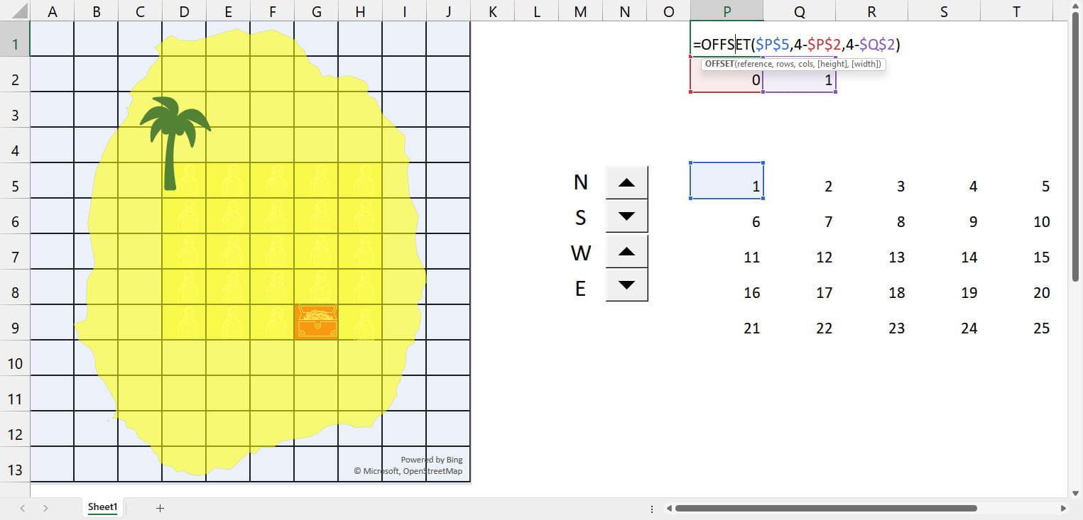
The simple form of OFFSET() has three arguments: a starting cell ($P$5), a number of rows to move up or down and a number of columns to move left and right. Positive numbers move down or right, negative numbers up or left. So, the value in P2 controls up and down, and the value in Q2 controls left and right. The reason to subtract each number from 4 is that we are using Spin Button form controls to change our values and these only work with positive numbers. Having the up arrow as ‘North’ is more intuitive than having it as South, so we need to decrease the value calculated in our function when we press the spin button up arrow, in order to increase the values in cells P2 and Q2.

As an example, if we start in cell P5, and press S twice and E three times, then P2 will contain 2, and Q2 will contain 1. So, we will start in cell P5, move 4-2=2 down to row 7 and 4-1=3 right to column S, selecting the value in S7 of 14. Our conditional format will then be applied to all the cells in our map grid of D5:H9, except the one that contains the value 14.

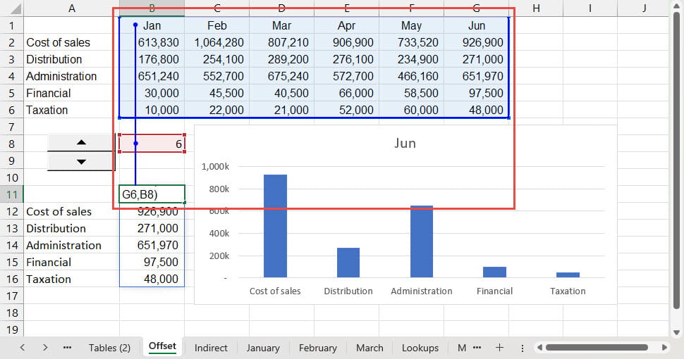
Having shown how OFFSET() works, it’s time to look at a more practical example. Here, we use OFFSET() in a similar way to allow the user to select the period that they want to chart:

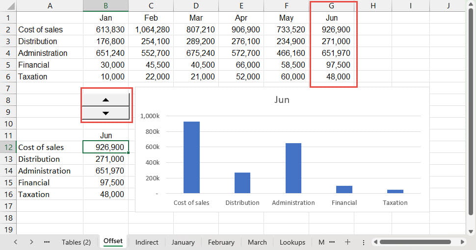
For example, cell B11 uses the following OFFSET() formula:

=OFFSET($B1,0,B$8)

We start in cell $B1, move no rows, but move the number of columns specified by the value in cell B$8, which is controlled by our Spin Button. Our other cells in B12 to B16 contain similar OFFSET() formulae so that, for each press of the up arrow or down arrow, we move right or left through our month columns. Our chart data source is set to A11 to B16, so our chart changes accordingly.

So what’s wrong with OFFSET()?

There are two main problems with the OFFSET() function. First of all, it is a ‘volatile’ function which means that it is calculated when there are any changes in the workbook. Most Excel functions are not volatile and so are only calculated when Excel knows that the change affects the relevant chain of calculations. The consequence of this is that using a large number of OFFSET() function formulae can negatively affect the speed of recalculating the workbook, whenever a change is made.

Possibly a more serious issue with OFFSET() concerns the dependent/precedent cell audit chain. Excel’s formula auditing tools are unable to correctly trace the precedent cells of a cell containing OFFSET(), or to show the OFFSET() function cell as being dependent on the cells that it actually refers to:

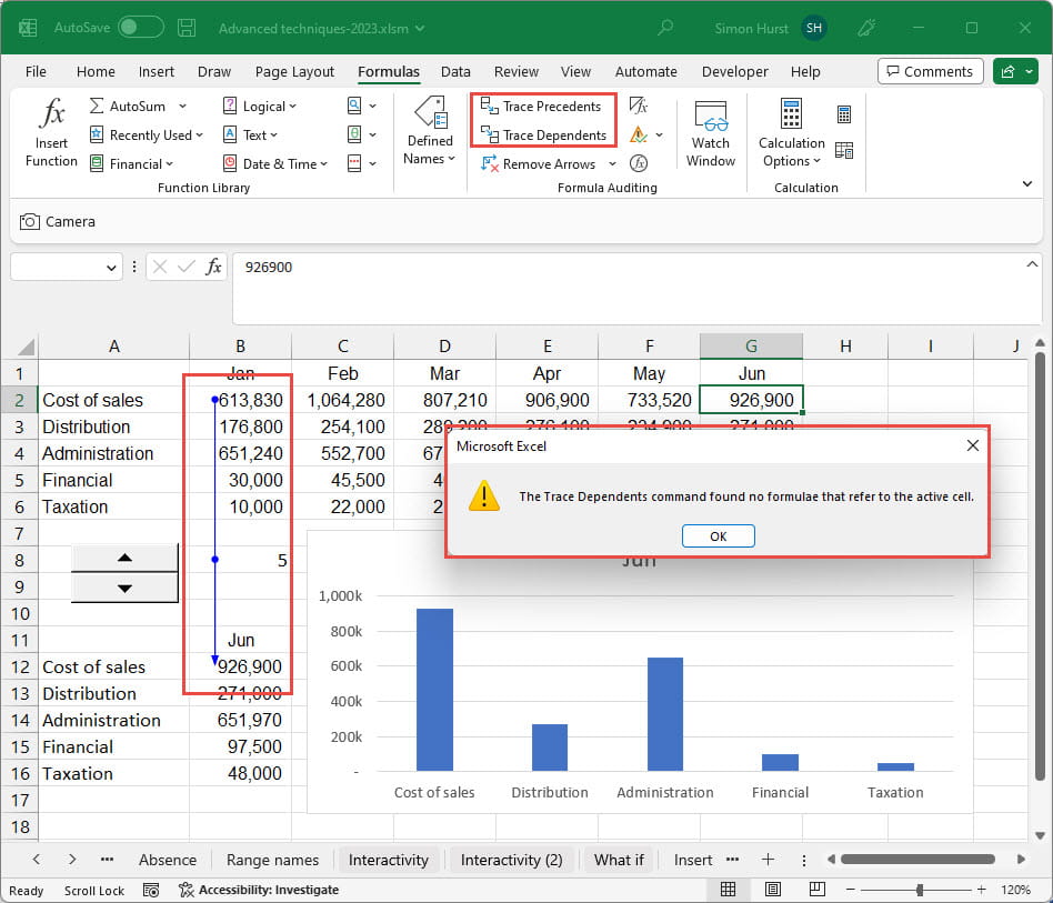
As you can see, for cell B12, containing our OFFSET() function, the trace precedent arrows do not refer to any of the cells used to calculate our chart values and, if we select G2 and try and trace dependents, Excel will suggest that none can be found.

In this case, the use of the INDEX() function would be a simpler alternative that would also preserve the audit chain:

=INDEX(P5#,5-P2,5-Q2)

INDEX() uses an array for its first argument, then a row position for its second argument and a column position for the third argument, returning the value at the intersection of the specified row and column.

Dynamic Array functions

It is often possible to avoid using OFFSET() by using the INDEX() function as we have seen, but this can be at the cost of needing to create a more complicated formula. However, In the brave new world of Dynamic Arrays, and with the recently released set of additional Dynamic Array functions, it is now much easier to find a way to replace OFFSET(). We need to make a small change in our Spin Button control as we will be choosing one of our six columns, rather than moving up to 5 columns from our first column:

Our formula is simpler than using the OFFSET() function and, because it uses a Dynamic Array, we only need to enter it in cell B11 and it will spill into our other cells:

=CHOOSECOLS(B1:G6,B8)

Our CHOOSECOLS() function has just two arguments in this case: the array from which to extract our column (or columns) and the index number of the column that we want to use. Our array could refer to an Excel Table so that it would adjust automatically as rows and columns are added to the data, giving it a further advantage over both the OFFSET() and INDEX() solutions.

Note that this would not have been such a complete solution to this particular problem before the recent change that allows an Excel chart to adjust dynamically as the dimensions of a Dynamic Array data source change.

Challenge

I know that many still find the OFFSET() function useful despite its issues. If you have a version of Excel that includes the new set of Dynamic Array functions, do you think that you will be able to replace all your uses of OFFSET(), or are there still situations when you feel that OFFSET() is still preferable or even essential? Let us know at excel@icaew.com.

Related links

• Excel Tip of the Week #112 - OFFSET
• INDEX() v OFFSET()
• Dynamic Arrays and Charts – bigger and better Excel dashboards await
• Charting with Dynamic Arrays
• Dynamic Arrays – still one leg short of a table?