This first post in the series Excel how to series will look at the Excel tools and techniques that help you accomplish a range of day-to-day Excel tasks more efficiently and effectively.
Introduction
Many of the areas covered will be well-known to experienced Excel users but it can still be useful to reflect on the importance of basic skills and techniques that can sometimes be incorrectly taken for granted.
As part of each article, we will be scouring the extensive Excel Community archive to provide links to additional details and ideas.
This first post will look at how to enter cell references in formulae as quickly and efficiently as possible.
Cell references
Almost all Excel calculations will use one or more cell references. There are many different ways to enter and edit cell references, some obvious, others less so. There is also one basic, but vital, Excel technique that can save you typing in hundreds of formulae and make your spreadsheets vastly more reliable at the same time.
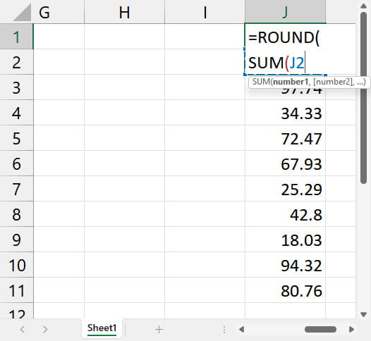
A cell reference can by typed in using the keyboard, such as = A 1, or just by typing = then clicking on the cell that you need to refer to. You can also use the keyboard cursor keys to move the selection to the required cell. This latter method can be useful when you can't click on the cell that you need to, because the current cell contents are in the way. In this example, we can't select cell J2 with the mouse, because our formula overlaps the cell. Instead, we can use the down cursor to select J2, and then hold down the Control and Shift keys together while using the down cursor again to select down to the last non-blank cell:
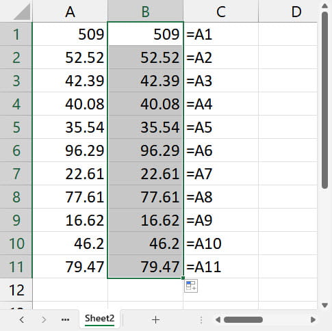
Perhaps the most significant way to speed up the entering of formulae is to understand how the dollar signs work in cell references to fix those references so that they don't change as they are copied to other cells. The key to understanding the dollar signs is to realise just what a cell reference like =A1 means. What it doesn't mean is =A1. We can prove this with the following simple example. If B1 was really a reference to A1, it wouldn't change when we copy it down to the other rows:
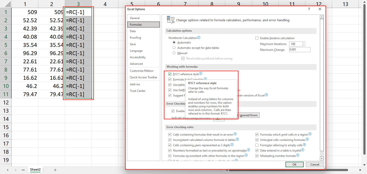
The apparent reference to A1 is, in fact, a reference to the relative position of A1 from the cell containing the formula. A1 is one cell to the left of B1, so the reference in cell B1 is actually a reference to the cell one column to the left. We can see this, and why it shows that our formula has been copied correctly, by changing our formula display to R1C1 style:
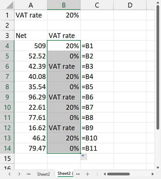
Of course, a lot of the time, this behaviour is exactly what we want, allowing us to copy formulae rather than enter each one individually. However, there are also many situations when we really do want to refer to a particular cell rather than a cell position. In this example, we have entered the VAT Rate of 20% in cell B1. We want to show this VAT rate for all of our values in A4:A14 but, if we just type =B1 into cell A4 and copy it down to the other cells, each of our cells will refer to the cell in the same column and 3 rows up: =R[-3]C:
To create our 11 formulae cells just using the default way of creating a reference could require the entry of 11 separate formulae. Not only does this have the potential to be vastly more time-consuming, but it also dramatically increases the likelihood of introducing errors. In addition, the increased number of individual formulae makes the resulting spreadsheet far more difficult to review.
The key to avoiding the individual formula catastrophe is to understand the use of the dollar signs in a cell reference to 'fix' all, or part of, that reference. Returning to our example, if we enter =B1 in cell B4 and then immediately press the F4 key on the keyboard, the reference to B1 will be changed to $B$1. This fixes the reference to the cell B1, wherever we copy the formula to. Here, we have copied our formula down to the other cells in column B:
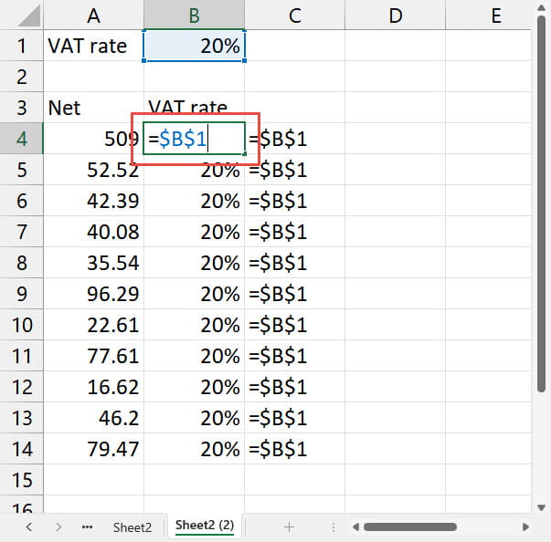
For the above, we used the F4 shortcut to go from B1 to $B$1. If we pressed F4 again, our reference would cycle to B$1, then to $B1, then back to B1. We can also just type in the dollar signs rather than using the F4 shortcut. There is a particular shortcut related to the use of F4. If you drag to create a reference to a range of cells such as A2:A5 then immediately press F4, the entire range, rather than just the reference to A5, will be made absolute:
=$A$2:$A$5
Whichever method we choose to enter our dollar signs, each dollar sign fixes the part of the cell reference that follows the dollar sign: B$1 fixes our reference to refer to row 1 wherever we copy it to, but the column reference, B, would change as we copied our formula to different columns. For $B1 this behaviour is reversed so that we can copy our formula to a different column and the reference will still refer to column B, but if we copy the formula to a different row, the row number will change.
Being able to use the dollar signs to fix elements of cell references will dramatically reduce the number of different formulae you need to type in; improve the consistency of your spreadsheets; make them easier to check and review and also make them significantly less error prone.
Related links:
Join the Excel Community
Do you use Excel in your organisation? Are you using it to its maximum potential? Develop your skills and minimise spreadsheet risk with our Excel resources. Membership is open to everyone - non ICAEW members are also welcome to join.

Archive and Knowledge Base
This archive of Excel Community content from the ION platform will allow you to read the content of the articles but the functionality on the pages is limited. The ION search box, tags and navigation buttons on the archived pages will not work. Pages will load more slowly than a live website. You may be able to follow links to other articles but if this does not work, please return to the archive search. You can also search our Knowledge Base for access to all articles, new and archived, organised by topic.

