Recently introduced in Excel, Dynamic Arrays allow a single formula to populate multiple cells. This brief introduction to how they work considers how they can speed up the creation of formulae and also enable an Excel formula to do more than would previously have been possible.
'How to' series
In this series we will be looking at the Excel tools and techniques that help you accomplish a range of day-to-day Excel tasks more efficiently and effectively.
As part of each article, we will be scouring the extensive Excel Community archive to provide links to additional details and ideas.
This is the story of the series so far:
- Excel how to: speed up entering formulae part 1 - using the dollar signs to fix all or part of a reference
- Excel how to: speed up entering formulae part 2 - using Range Names to make formulae easier to enter and understand
- Excel how to: speed up formulae - using Excel tables – creating dynamic references by referring to Table columns and using Table structured references to make formulae easier to understand
- Excel how to: speed up formulae - using Excel tables part 2 – adding calculated columns to an Excel Table
Dynamic Arrays
Dynamic Arrays were introduced relatively recently and are available in Excel for Microsoft 365 and Excel 2021. They represent a very significant change to the way that Excel formulae work. A single formula can now ‘spill’ into as many adjacent cells as are necessary to represent the cell range referred to. This means that the same formula will behave differently in versions of Excel without the new feature compared to the current version.
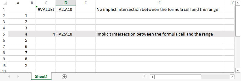
Before the introduction of Dynamic Arrays, just referring to a range of cells such as =A2:A10 would generate a #VALUE! error (as long as there is no ‘implicit intersection’ between the range and the formula cell):
With Dynamic Arrays, Excel would recreate the contents of A2:A10 in adjacent cells starting with the formula cell:
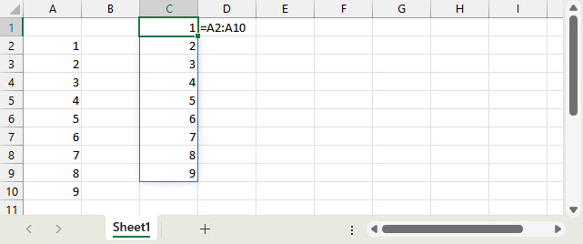
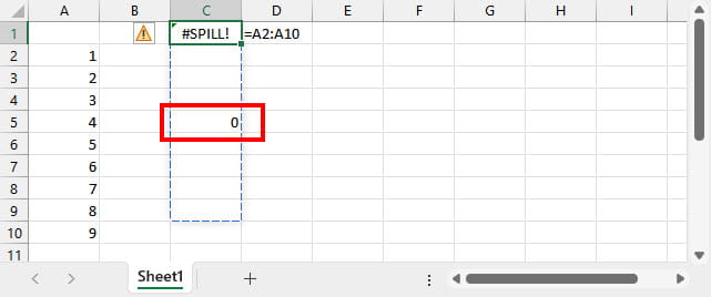
Examining the contents of the cells will show that cell C1 contains our formula and can be edited. Cells C2 to C9 will display our =A2:A10 formula as greyed out and the formula in these cells cannot be edited. Obviously, there is a potential issue with a formula spilling into cells that already contain content. If existing cell contents are in the way, the formula will not spill at all, and a #SPILL! error will be generated in the formula cell.
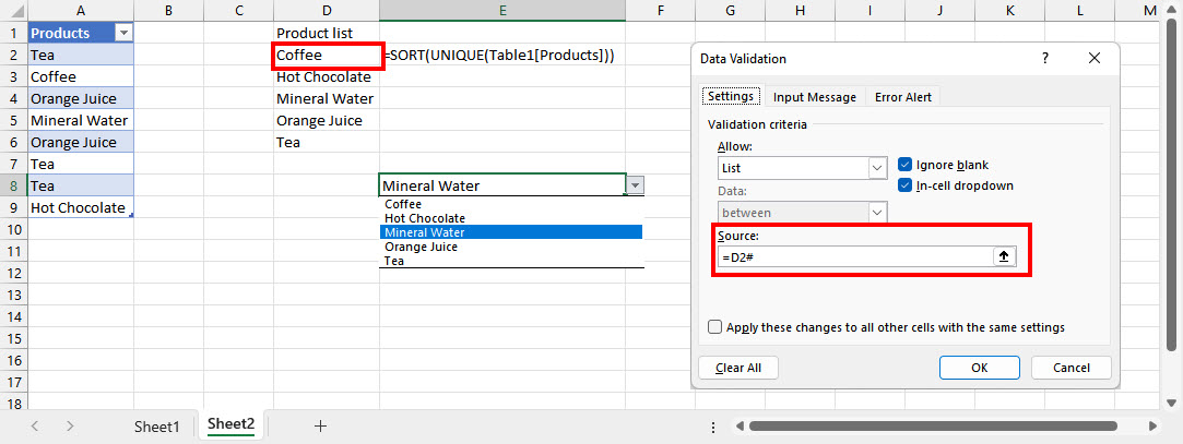
As well as the way in which Dynamic Arrays change how references to cell ranges work, when Dynamic Arrays were first introduced, a set of functions was also added to work with them. For example, the SORT() function allows the result of a Dynamic Array reference to be sorted and the UNIQUE() function can remove duplicates. A practical use of these two functions would be to create a sorted list, suitable as the source of a Data Validation dropdown:
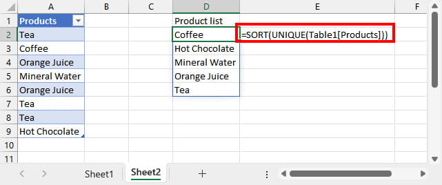
In this example, our Dynamic Array reference refers to a Table column and returns a list of the items in our Products Table in alphabetical order and with duplicates removed. Unfortunately, although Dynamic Arrays can refer to Tables, they cannot themselves be part of a Table, which can make it more difficult to refer dynamically to the result. In some cases, a special operator can be used instead. Adding the # character after a reference to the top-left cell of a Dynamic Array will create a reference to the entire array. Here we can see it used as part of a Data Validation list source:
Further Dynamic Array functions have been added to Excel for Microsoft 365 in the last few months allowing Dynamic Arrays to be ‘stacked’ and ‘shaped’.
In terms of speeding up the entry of Excel formulae, Dynamic Arrays can replace multiple, complex formulae with a single, simple formula. In this example, we have used a single formula to round the individual values in a Table column and sum the result:

This is possible in versions of Excel before Dynamic Arrays were introduced, but would require the use of fragile, and generally not well-known, array formulae created through the use of the Control+Shift+Enter key combination, or a ‘wrapper’ function like SUMPRODUCT().
Understanding how Dynamic Arrays and Dynamic Array functions work can not only allow formulae to be created more quickly, but can also allow an Excel formula to do something dynamically that would have needed manual intervention previously, such as appending multiple ranges to create a single range.
It’s well worth exploring Dynamic Arrays further, and a forthcoming Excel Community webinar will do just that:
Related links:
Archive and Knowledge Base
This archive of Excel Community content from the ION platform will allow you to read the content of the articles but the functionality on the pages is limited. The ION search box, tags and navigation buttons on the archived pages will not work. Pages will load more slowly than a live website. You may be able to follow links to other articles but if this does not work, please return to the archive search. You can also search our Knowledge Base for access to all articles, new and archived, organised by topic.

