Introduction to power pivot data analysis expressions (DAX): Part 2

Northwind includes a set of sales invoice data. This data includes the amount of each invoice line and the name of the salesperson responsible for the sale as well as the order date relating to each invoice. We are eventually going to create a PivotTable that will compare the sales for each year with sales for the previous year and then work out a budget.

DAX CALCULATE() in practice

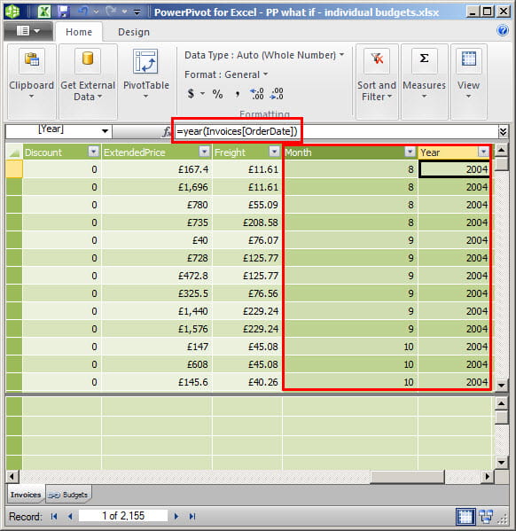
Having got the background of DAX out of the way in part 1, we will now consider the use of the CALCULATE() DAX expression in practice. One of the things that you can’t do in PowerPivot is to group existing fields within the PivotTable itself – this is a particularly useful technique for working with dates, when you might want to report on sales by month or by year, but your dates are recorded day by day. Here, to overcome this shortcoming of PowerPivot, we have used the DAX YEAR() and MONTH() functions to add Year and Month columns to our Northwind invoice data:

Now we will move to our PivotTable itself and create a Measure. We want our DAX measure to calculate the sales for the previous year. Date calculation functions form the majority of the DAX functions available and allow for a wide range of different calculations based on the value of date fields. We will use the comparatively simple PREVIOUSYEAR() function.

Where DAX YEAR() works in a familiar way to the worksheet YEAR() function, PREVIOUSYEAR() is much more like a database operation than a cell function. First of all, it is not intended to return a single value, but instead a range of dates to be used as a database criterion. It is also not designed to have a single value as an argument, but instead uses a ‘column’. In effect, we are creating a criterion for a column of data in our Invoices table.

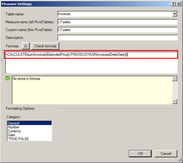
The next thing to understand about DAX used as a measure is that you are not working with a single cell but a table of values. This means that, in a similar way to an Excel reference, you must use an appropriate aggregate function – usually SUM() – to turn your set of individual values into a single value. CALCULATE() lets us combine our SUM() with the date criterion provided by PREVIOUSYEAR() to generate a total of all our invoices for the previous year:

We can add a new measure by choosing New Measure from the Measures group of the PowerPivot ribbon. We can then give it a name: ‘LY sales’ in this case.

Our SUM() function totals the values from the ExtendedPrice column of our Invoices table. CALCULATE() applies one or more filters to the Invoices table to change the result of the SUM(). In this case we have just applied one filter – we have used PREVIOUSYEAR() to restrict the rows included in our SUM() to those which have a date in the previous year.

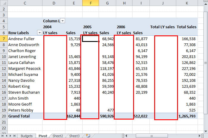
Now let's use our Year column as a row heading and add our LY Sales measure to see the values for the current and previous years:

Our LY sales columns are all blank. This is because CALCULATE() adds filters to create the required SUM(), it doesn’t override existing filters. As we discussed in part 1, thinking in database, rather than worksheet, terms, each cell has several filters applied to it already. For example, G7 is filtered to the Salesperson ‘Andrew Fuller’ (Row label) and the year 2005 (Column label) as well as the PREVIOUSYEAR() filter applied by CALCULATE(). This is the problem: for a transaction to be included in our SUM() it must survive all three filters. Unfortunately, this means it needs to be in both 2005 and the previous year, 2004, which is impossible –hence the blank columns.

Again, the answer is to think in database terms rather than worksheet. In a database query, we could add an additional criteria row which works as an ‘OR’ filter allowing rows through the filter that other criteria in the same column would reject. We can do something similar within our CALCULATE() function using ALL(). ALL() allows us to ignore any filters applied by the PivotTable on a particular column. In this case we need to ignore the PivotTable filter on the Year column:

=CALCULATE(SUM(Invoices[ExtendedPrice]),PREVIOUSYEAR(Invoices[OrderDate]),ALL(Invoices[Year]))

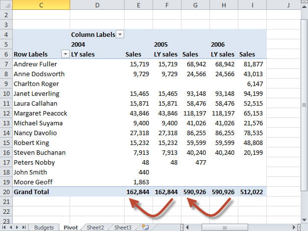
By removing the Year criteria, our CALCULATE() formula now includes values for each of our columns:

Our problems are not quite over yet – if you look carefully at the totals for 2004 sales and 2005 LY sales you will see that they are the same, but that the individual salesperson details for the 2005 LY sales omit the amounts for those salespersons with no sales in 2005. This is because, irrespective of including all years, there are no values in Invoices[OrderDate] for PREVIOUSYEAR() to work out the previous year. One answer is to create a table containing all possible dates. We will look at this in the next part before we go on to consider budgets and variances.

Office Tips

Simon has included many useful Excel tips in the 'Lunchtime Learning' section of his website.

Trademark acknowledgements

Excel is a registered trademark of Microsoft inc.

Screen shots reprinted by permission from Microsoft Corporation.