You can use your favourite search engine to find methods, which usually culminate in opaque user defined functions, grid computations similar to depreciation calculations, or else brute force VBA. Indeed, often you will find self-appointed sages decreeing that you have to resort to these methods because a formulaic method is “just not possible”.

Hogwash.

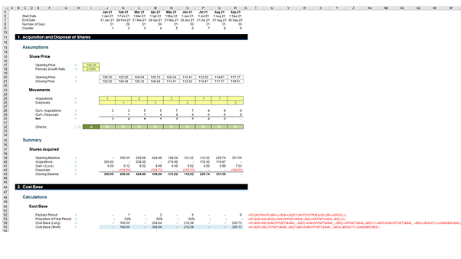
Consider the following example. Imagine you decided to dabble in buying and selling shares:

In the attached Excel file, I have assumed:

• the opening price of shares is $100 per share
• the share price grows 2% each time (there is no need to assume a uniform rate; this makes no difference to the mechanics of the cost calculation)
• three shares are purchased in the first period (Jan 21) for $100 each
• two shares are purchased in the third period (Mar 21) for $100 x (1 + 2%)2 = $104.04 each
• two more shares are purchased in the fifth period (May 21) for $108.24, and then one each in July and August for $112.62 and $114.87 respectively
• these shares are sold: one in Feb 21, three in April, two in June and the final three in September
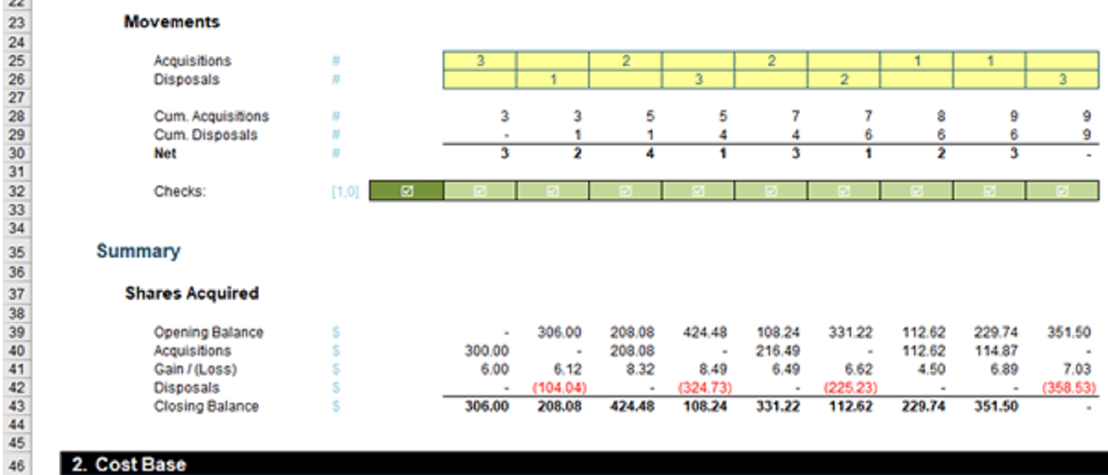
• rows 28 and 29 (above) provide cumulative totals of the purchases and disposals respectively
• the error check in row 32 merely ensures you don’t dispose of more shares than you own
• rows 39:43 in the image create a control account which for the dollar amounts, which shows the shares bought at opening prices, sold at closing prices and the interim gains / (losses) so that once all shares are disposed of the closing balance is once again nil
• the attached Excel file may be reviewed to see how these formulae work. However, that is not the main focus of this article.

This sets the scene, and is something that could easily be envisaged in the real world. Row 42 (Disposals) depicts the sales proceeds. However, what are the associated costs of goods sold? We could use the averaging method from last time, but in many tax regimes around this world, this option is not allowed.

Instead, many such regimes require a First In, First Out (FIFO) basis of attributing the costs to determine the taxable profit. If you think about it, that makes sense – provided you are the tax authority or a beneficiary thereof! If share prices are going up, this approach will maximise the Net Present Value of your profits – i.e. more tax to pay in real terms!

This provides not only a tax planning, but also a computational, headache. You want to find a way to calculate this fee for your FIFO fumbles (see where my title comes from now, dear editor..?).

This is the problem:

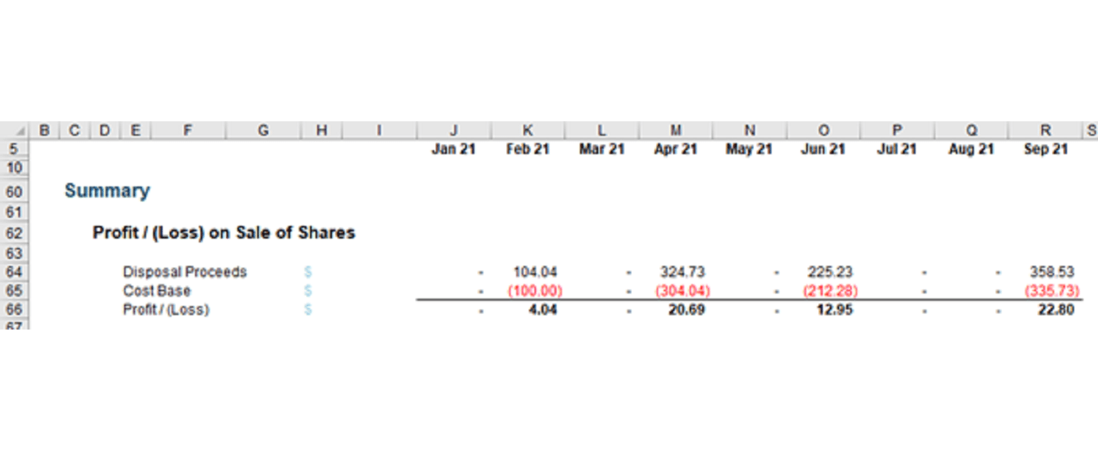
• first disposal in February is simply $100, being the cost of one of the initial three purchases the month before
• however, the second disposal of three shares is $304.04. This is because the other two shares purchased for $100 in January are sold, plus one of the March acquisitions at $104.04, which equals (2 x $100.00) + $104.04 = $304.04
• the third disposal in June is $212.28. This is the other share acquired in March for $104.04 plus one of the two May purchases of $108.24, and $104.04 + $108.24 = $212.28
• the final disposal in September is $335.73. This represents the other May purchase ($108.24), combined with the July ($112.62) and August ($114.87) acquisitions. This adds up to $108.24 + $112.62 + $114.87 = $335.73.

Once you get your head around the concept, it makes perfect sense. The question is, how on Earth do you model it? And this is where our internet experts resort to user-defined functions, VBA and witchcraft / wizardcraft (no sexism here, thank you).

The computations may not be the most transparent I have ever written, but it can be calculated in just THREE lines, viz.

Did you say three calculations, Liam? I clearly see four. Yes, that’s true, but the third formula (row 54) is only included in order to explain the shorter variant (fourth line, row 55). And be careful Liam, holding discussions with yourself is the second sign of madness*.

(*N.B. First sign of madness is asking, “what’s the first sign of madness?”.)

For those of us who are not emmetropians (look it up, it’s your word for the day!), let’s go through each of those last four formulae in turn.

Row 52, Payback Period, has inquired about the final period required that acquired shares (sorry, I couldn’t resist that sentence: you wish to criticise, you write these articles!). In English, this denotes the final period where shares were purchased, in order to service the share disposal figure for that period. To be clear:

• first disposal in February is simply period 1 (Jan 21), as only one of the three shares purchased in January is needed to service the disposal
• the second in April returns period 3. This is because the other two shares purchased in January (period 1) do not fully service the requirement of three shares. Therefore, one of the March (period 3) acquisitions is needed too
• the third disposal in June returns period 5. This is the because not only is the other share acquired in March (period 3) sold, but also one of the May (period 5) shares is disposed of as well
• the final disposal in September returns period 8. This is because all the remaining shares are now disposed of, with the last acquisition made in August (period 8)
• the other periods return zero (-) as no “payback” is made in these months.

To find the first period where the cumulative total of acquisitions (row 28) is equal to or exceeds the number of disposals required, we can use the formula

=MATCH(TRUE,$J28:J28>=J$29,0)

in cell J52 and copy it across.

MATCH with type 0 for the third argument simply seeks out the first occasion of TRUE in the vector specified by the second argument (a vector is simply a row or column of cells). For example, the formula in cell O52 would be

=MATCH(TRUE,$J28:O28>=O$29,0)

The argument $J28:O28>=O$29 would return

{J28>=O$29, K28>=O$29, L28>=O$29, M28>=O$29, N28>=O$29, O28>=O$29}

which would equate to

={FALSE, FALSE, FALSE, FALSE, TRUE, TRUE}

The first TRUE occurs in position 5, hence O52 returns the value 5. However, the formula is more complex than this. That’s because life is never that simple!

For a start, the formula in cell J52 is

=MATCH(TRUE,$J28:J28>=J$29,0)

This is the equivalent of

=MATCH(TRUE,$J28>=J$29,0)

The second argument is not a vector; it is merely one cell compared with another. MATCH doesn’t like this. Therefore, whether the result is TRUE or FALSE, this formula will always return #N/A – the formula is not applicable. We need to account for this:

=IF(J$9=1,(J$28>=J$29)*1,MATCH(TRUE,$J28:J28>=J$29,0))

This “wraps up” our formula by checking if it is the first month (row 9 is a period counter, so J$9=1 is checking whether it is the first period).

The next problem is that if we have an instance where there is no payback (e.g. assume the checks in row 32 are breached), the formula will again return #N/A – this time to indicate that the payback period is not available. This can be countered easily:

=IFNA(IF(J$9=1,(J$28>=J$29)*1,MATCH(TRUE,$J28:J28>=J$29,0)),)

This will just replace #N/A with zero (0), as nothing is specified after the final comma (IFNA simply checks whether a formula specified in the first argument returns #N/A and specifies what to do in this instance in the second argument).

Finally, to ensure that the formula only calculates in periods where there are disposals, one further modification is made:

=IF(J26,IFNA(IF(J$9=1,(J$28>=J$29)*1,MATCH(TRUE,$J28:J28>=J$29,0)),),)

This just checks that J26 is non-zero. This provides us with a hideous nested IF formula, but one that does indeed specify the appropriate payback period:

=IF(J26,IFNA(IF(J$9=1,(J$28>=J$29)*1,MATCH(TRUE,$J28:J28>=J$29,0)),),)

This then begs the question, so why did we need this? It’s because the next step is to work out the total costs for all to disposals up to this point:

• first disposal in February needs to be serviced by acquisitions in January
• disposals in February and April are serviced by acquisitions in January and March
• disposals in February, April and June are serviced by acquisitions in January, March and May
• all disposals (up to September) are serviced by all the acquisitions up to and including August.

Consider the second and subsequent sales of shares:

• the disposals in February and April use all of January’s acquisitions and a proportion of March’s
• the disposals in February, April and June use all of January’s and March’s acquisitions and a proportion of May’s
• the disposals up to and including September use all of the purchases made up to July and a proportion of August’s (which just so happens to be 100%).

Therefore, we have a plan of action. To work out the costs up to and including a particular sale:

• sum all the acquisition costs for the period prior to the payback period (all of these costs will have been consumed, as explained above)
• for the breakeven period, calculate the proportion used.

This is why I have computed the breakeven period. Now, I need to work out the proportion used in this identified cut-off (payback) period. To do this, I need to use two of my most frequently used functions, namely MOD and OFFSET.

Refresher on MOD

The MOD function, MOD(number, divisor), returns the remainder after the number (the first argument) is divided by the divisor (the second argument). The result will have the same sign as the divisor.

For example, MOD(47,7) equals 5, since 47 divided by seven (7) is 6 remainder 5. Remainders can vary from zero to any number strictly less than divisor. The trick I will employ uses MOD(calculation, 1), which will calculate any non-integer component of a calculation (i.e. a value greater than or equal to zero [0] and strictly less than one [1] for a positive divisor). This forms the crux of calculating the payback period proportion.

Refresher on OFFSET

Regular readers will recognise I use this function all the time! The syntax for OFFSET is as follows:

OFFSET(reference, rows, columns, [height], [width])

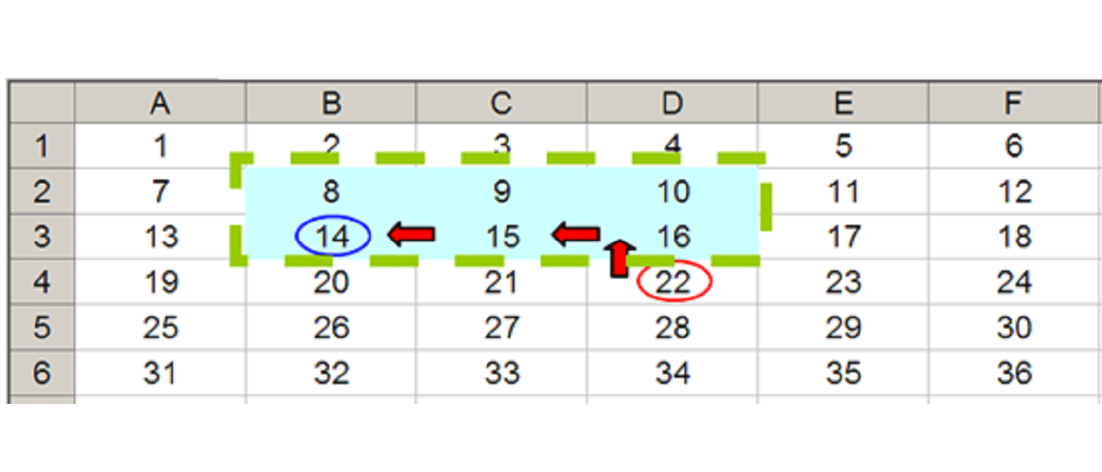
The arguments in square brackets (height and width) may be omitted from the formula (they both have a default value of 1 which is explained further, below). In its most basic form, OFFSET(reference, x, y) will select a reference x rows down (-x would be x rows up) and y columns to the right (-y would be y columns to the left) of the reference reference. For example, consider the following grid:

OFFSET(A1,2,3) would take us two rows down and three columns across to cell D3. Therefore, OFFSET(A1,2,3) = 16, viz.

OFFSET(D4,-1,-2) would take us one row up and two rows to the left to cell B3. Therefore, OFFSET(D4,-1,-2) = 14, viz.

OFFSET may also take advantage of the height and width arguments. If we extend the above formula to OFFSET(D4,-1,-2,-2,3), it would again take us to cell B3, but then we would select a range based on the height and width parameters. The height would be two rows going up the sheet, with row 14 as the base (i.e. rows 13 and 14), and the width would be three columns going from left to right, with column B as the base (i.e. columns B, C and D). 

Hence, OFFSET(D4,-1,-2,-2,3) would select the range B2:D3, viz.

Note that OFFSET(D4,-1,-2,-2,3) = #VALUE! where dynamic arrays are not recognised, since Excel cannot display a matrix in one cell, but it does recognise it. However, if after typing in OFFSET(D4,-1,-2,-2,3) we press CTRL + SHIFT + ENTER, we turn the formula into an array formula: {OFFSET(D4,-1,-2,-2,3)} (do not type the braces in, they will appear automatically as part of the Excel syntax). This gives a value of 8, which is the value in the top left-hand corner of the matrix, but Excel is storing more than that. This can be seen as follows:

• SUM(OFFSET(D4,-1,-2,-2,3)) = 72 (i.e. SUM(B2:D3))
• AVERAGE(OFFSET(D4,-1,-2,-2,3)) = 12 (i.e. AVERAGE(B2:D3)).

It is SUM(OFFSET) and being able to vary a reference based upon a given number of columns that I intend to use here.

Returning to FIFO

In cell J53, consider the formula:

=MOD((J$29-OFFSET($I$28,,J$52))/OFFSET($I$25,,J$52),1)

OFFSET($I$28,,J$52) uses the OFFSET function to find the payback period’s cumulative number of acquisitions. This is why the reference cell is I28 – moving one column to the right provides January’s details (period 1), moving two columns to the right provides February’s details (period 2), and so on. The number of columns to the right (J$52) is given by the identified payback period number.

J$29-OFFSET($I$28,,J$52) thus calculates the payback period’s cumulative acquisitions from the current period’s cumulative disposals. This should always provide a non-positive number, which is intentional, to get the correct proportion. In absolute terms, this number should also be less than or equal to the number of purchases made in the payback period – as this is the definition of the payback period.

OFFSET($I$25,,J$52) is the total number of purchases (acquisitions) made in the identified payback period. Therefore, using the trick discussed above when introducing OFFSET,

=MOD((J$29-OFFSET($I$28,,J$52))/OFFSET($I$25,,J$52),1)

calculates the required proportion.

Since we only want this formula to calculate when there has been a sale (disposal, as shown in row 26) and when a payback period (row 52) has been calculated, the formula is placed inside an IF statement, viz.

=IF(J$26*J$52,MOD((J$29-OFFSET($I$28,,J$52))/OFFSET($I$25,,J$52),1),)

This is the formula in row 53. Just take note of one important point here: if there is no remainder (i.e. the value is zero [0]), this formula will result in zero (0). Strictly speaking, the proportion used in the payback period would be 100% though, not zero, so we will need to make an adjustment in this instance. I will revisit this scenario shortly.

Now comes the fun part (!).

To calculate the cost base used for all disposals, this will equal:

• the sum all the acquisition costs for the period prior to the payback period (as explained earlier). This will be given by the formula
  
  =SUM(OFFSET($I$40,,,,J$52))

• this sum needs to be modified though if 100% of the costs are used in the payback period (i.e. the next period needs to be included too):
  
  SUM(OFFSET($I$40,,,,J$52+(J$53=0)*1))

• for the breakeven period, we will need to calculate the proportion used, which is calculated in parts. Consider
  
  = SUM(OFFSET($J$40,,,,J$52))-SUM(OFFSET($I$40,,,,J$52))

which simply derives the acquisition costs for all periods up to and including the payback period less the acquisition costs for all periods prior to the payback period, i.e. just the payback period’s total acquisition costs, less

OFFSET($I$40,,J$52)*(1-J$53)

which is the unused proportion in the payback period. Adding these two parts together will give us what we need.

Still with me? No, I’m not either. However, if we combine these calculations, we obtain the total costs for all disposals so far:

=SUM(OFFSET($J$40,,,,J$52))-SUM(OFFSET($I$40,,,,J$52))-OFFSET($I$40,,J$52)*(1-J$53)+SUM(OFFSET($I$40,,,,J$52+(J$53=0)*1))

We now need to calculate the costs just for the disposal in that period alone, which is the total costs calculated, less all the costs calculated for earlier periods, i.e.

=SUM(OFFSET($J$40,,,,J$52))-SUM(OFFSET($I$40,,,,J$52))-OFFSET($I$40,,J$52)*(1-J$53)+SUM(OFFSET($I$40,,,,J$52+(J$53=0)*1))-SUM($I$54:I$54)

Since we again only want this formula to calculate when there has been a sale (disposal, as shown in row 26) and when a payback period (row 52) has been calculated, the formula is once more placed inside an IF statement, viz.

=IF(J$26*J$52,SUM(OFFSET($J$40,,,,J$52))-SUM(OFFSET($I$40,,,,J$52))-OFFSET($I$40,,J$52)*(1-J$53)+SUM(OFFSET($I$40,,,,J$52+(J$53=0)*1))-SUM($I$54:I$54),)

This is the formula in cell J54:

=IF(J$26*J$52,SUM(OFFSET($J$40,,,,J$52))-SUM(OFFSET($I$40,,,,J$52))-OFFSET($I$40,,J$52)*(1-J$53)+SUM(OFFSET($I$40,,,,J$52+(J$53=0)*1))-SUM($I$54:I$54),)

Eagle-eyed readers will spot this is more complex than it needs to be, which is why this is called the “Long” formula. The expression

SUM(OFFSET($J$40,,,,J$52))-SUM(OFFSET($I$40,,,,J$52))-OFFSET($I$40,,J$52)*(1-J$53)

may be simplified to

OFFSET($I$40,,J$52)*J$53

which is quite a simplification! Therefore, using this substitute provides us with the “Short” formula in cell J55:

=IF(J$26*J$52,OFFSET($I$40,,J$52)*J$53+SUM(OFFSET($I$40,,,,J$52+(J$53=0)*1))-SUM($I$55:I$55),)

Clear as mud? Nonetheless, this provides us with the correct cost base for the period, without fancy footwork using user defined functions, grid algebra or VBA. From here, it is simple, to work out the profit assessable to tax:

It’s not pretty, but it is FIFO.

Word to the Wise

Apologies, it’s not the simplest concept we have ever discussed, but this is a common problem in financial modelling. I wanted to show it for this reason – and because so many naysayers you cannot do this formulaically!

Some more advanced readers might consider using SUMPRODUCT and INDEX instead. This is because SUMPRODUCT cross-multiplies costs, and INDEX is not a so-called volatile function, which means it does not recalculate every time you press ENTER.

Given the name of my company is SUMPRODUCT, rest assured, dear reader, I have plenty of time for this function, but sometimes it slows down calculations, certainly compared to SUM. Similarly, OFFSET may be volatile, but it also often calculates more quickly than INDEX, especially given you would need multiple INDEX expressions. In larger models, you will find my formulae will calculate more quickly than using these alternatives – but it’s not wrong to use them instead.
It would be a boring world if we all thought the same.