Economic life modelling

The definition of economic life is stated as the timespan over which the annual cost of owning and operating a non-current asset (held for continuing use in the business) is minimised. The economic life of such an asset can be a function of factors such as physical wear and tear, usage and technological obsolescence.

In order to establish what constitutes minimum costs, I want to consider not only the costs incurred but the timing of them too – so we need to dust down discounted cash flows.

The easiest way to explain this is with an illustration. Assume I have the following forecast cost data:

For this non-current asset, I have three cost categories, forecast for each of the next eight years (you may need to project further in real life).  Do note that the Purchase Price is the cost to buy a new, replacement asset in x years from now – not the purchase price to buy the asset now. That figure is both sunk and / or decision irrelevant as we are assuming we already have the asset.

I assume Maintenance Costs will be incurred each year.  To keep the discounted cash flow simple, I will assume the costs are incurred at the end of each period too (not an unreasonable assumption to make as businesses will often try to keep their costs to a minimum and tend to delay costs where they can).

Assuming we replace this asset after eight (8) years, a discounted cash flow financial appraisal would look something like this:

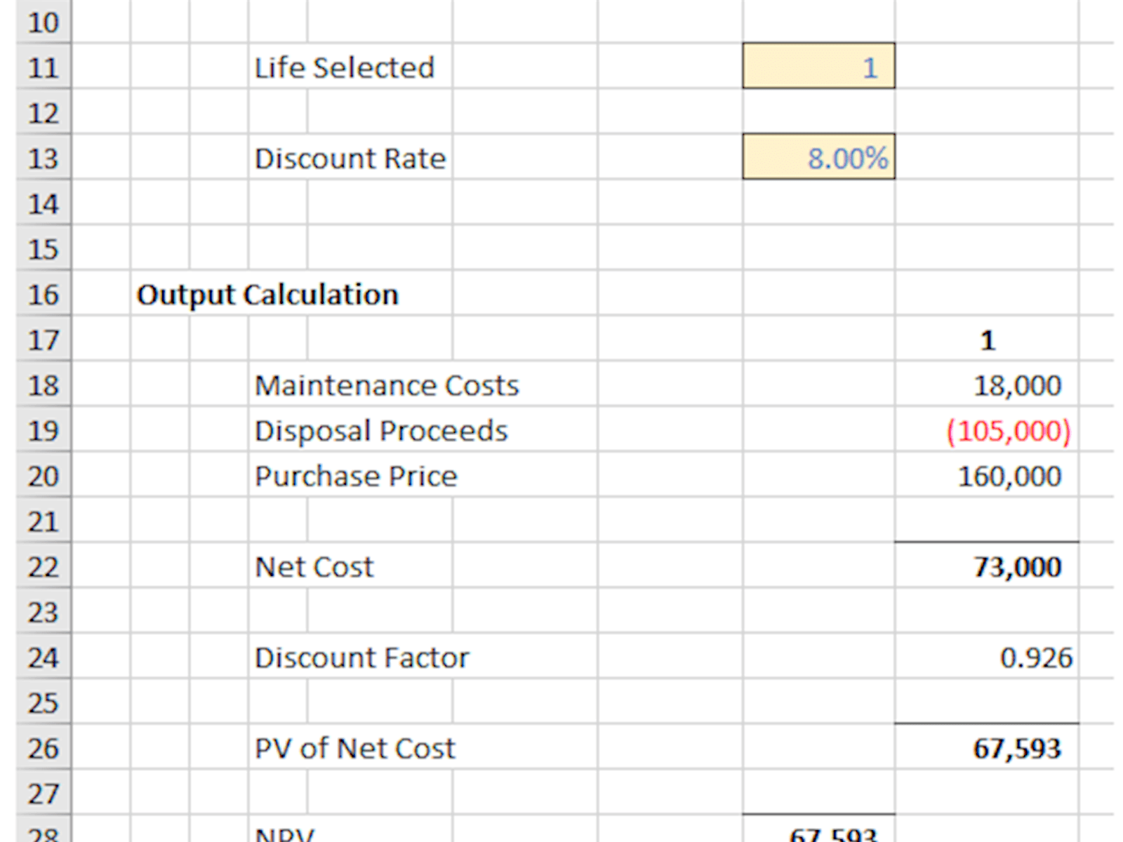
Do note that I ignore tax, as this would be an assumed constant and again, is decision irrelevant. What you might see in these straightforward calculations is several IF statements that cut off costs after so many periods, or only display them for a particular period. That is so I may vary the life assessed. For example, this would be the Net Present Value (NPV) for one year:

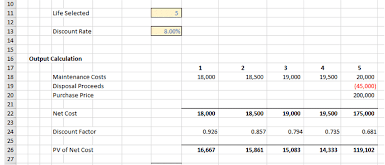
For five years, the calculation would be:

Note I calculate the discounted cash flows from first principles – there are too many mistakes made when you use Excel’s built-in NPV and XNPV functions. It’s also easier for end users to follow intuitively.

Obviously, the costs appear to increase each year, as there will be additional Maintenance Costs, Disposal Proceeds will reduce and the Purchase Price will increase. On that basis, we should replace assets once every picosecond, but that’s not exactly viable. Besides, it would be wrong.

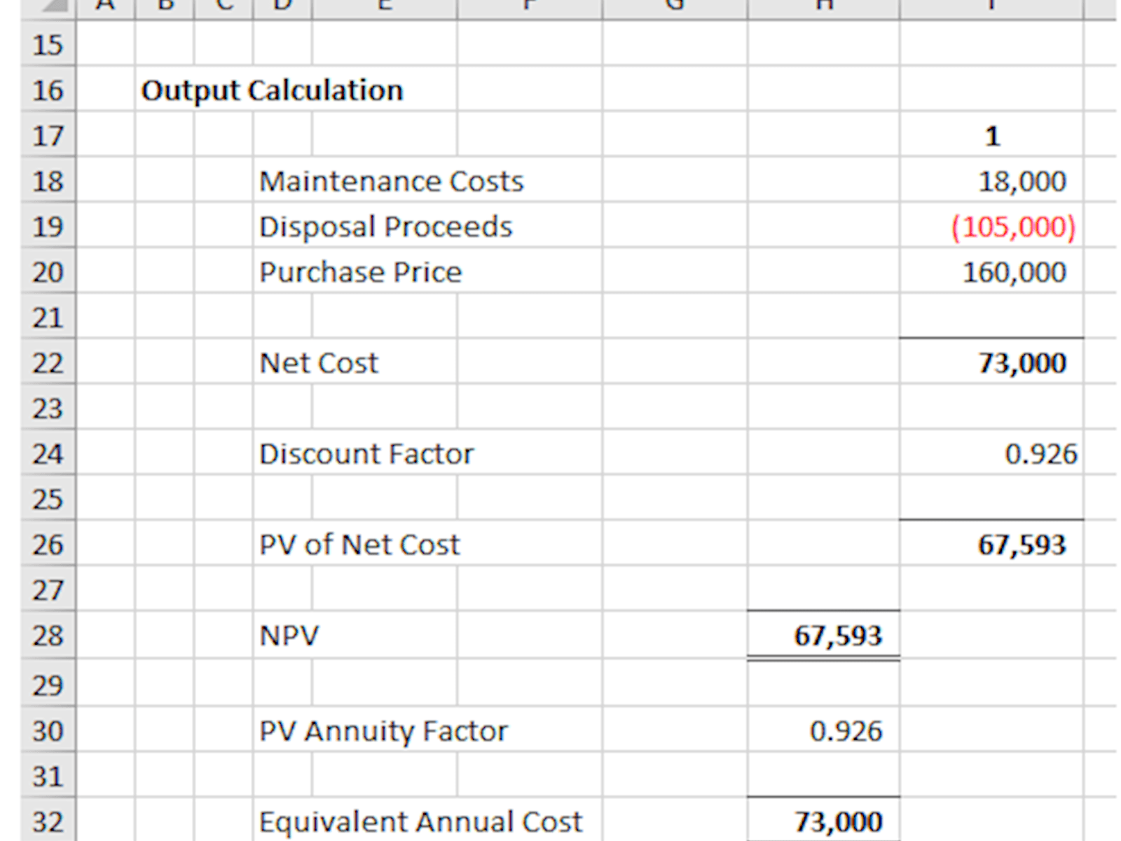
We need to calculate the average annual cost. Simply dividing by the number of periods would be incorrect as we are discounting the cash flows. We need to take this into account. Therefore, we weight this average by diving by the sum of the discount factors instead (known as the cumulative discount factor):

Our initial eight-year appraisal would then become:

whereas the one-year assessment would be:

Clearly, eight years would be a better bet than one year, on this basis.

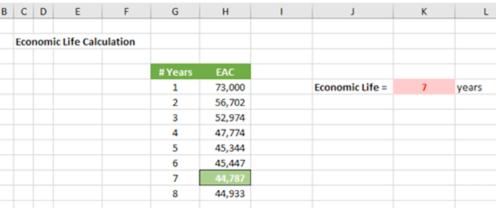
Rather than estimate the economic life by performing a “manual goal seek”, I can derive the optimum figure using a one-dimensional column Data Table (ALT + D + T):

I have put the formula =H28 in the hidden cell H38, then highlighted the range G38:H46 before creating the Data Table. This shows that for the costs forecast, the economic life for this asset should be seven (7) years, viz.

With the correct set-up, this economic life verification becomes trivial and should therefore be performed at least once a year, in order to confirm the appropriate accounting policies, etc.