Familiarity with the basic idea of discounted cash flows is presumed for this blog.

Net present values

Discount rates aren’t too complicated to calculate directly in Excel, but to save time, there are a couple of simple functions available to do the calculations in a single step. These let you take a series of cash flows, a discount rate, and simply output the final net present value figure.

Let’s start with the simplest function, NPV:

=NPV(discount rate, values)

Discount rate is the applicable discount rate, expressed as a percentage
Values is a list of the cash flows to be discounted – these can be in a row or in a column

This function just applies the stated discount rate to each value – once to the first item, twice to the second, and so on – and then adds the total. In other words, the discount rate is presumed to be per each period, and each successive value is one period after the next. Note that all the values are discounted i.e. it is presumed that the first cash flow occurs at the end of the first period. If you have any undiscounted cash flows, i.e. cash flows at the beginning of the first period, then you need to add those to the result of the NPV function.

XNPV is much the same, except that it can handle uneven payment schedules. You need to provide dates for each cash flow:

=XNPV(discount rate, values, dates)

Dates is the new argument here – this must be a range of dates the same size as the values range

Note that XNPV will discount to the first date in the given date series – i.e. it will not discount the first cash amount at all. If you instead want to discount to today’s date or some other earlier date, add a column at the beginning with that date and £0 associated cash flow. 

Naturally, XNPV is more precise than just NPV. Using the same data as above, XNPV gives us £5,568 – £13 lower than the straight NPV calculation.

There is a demonstration of both methods, along with a direct calculation showing how each works, in this file

Internal rates of return

You can find internal rates of return – that is, the discount needed for a £0 NPV – for many discounting calculations using Goal Seek (see TOTW #250 for more on that). Goal Seek works through iterative trial-and-error to solve these kinds of problems, but you can also use the IRR and XIRR functions to do the same. Note however that these functions also calculate iteratively – that is, they’re not precisely mathematical, and may sometimes fail or give slightly inaccurate answers.

Once again, we’ll start at the simpler function, IRR:

The syntax is very simple:

=IRR(values)

Just like NPV, this presumes that discounting starts straight away, so that the first amount is discounted once, the second twice, and so on.

There’s actually an optional second input – guess. You can use this to “seed” the starting value for the iterative calculation, which can improve accuracy and stability. Sometimes there are multiple values that lead to a 0 NPV. Inputting a guess value can help if the function doesn’t behave as you expect. If you don’t include one, Excel uses 10% by default.

XIRR is the date-specific version:

=XIRR(values, dates)

The optional guess input is also available. XIRR calculates the same way XNPV does – i.e. assuming that the first amount is not discounted, and discounting all other cash flows with respect to that date.

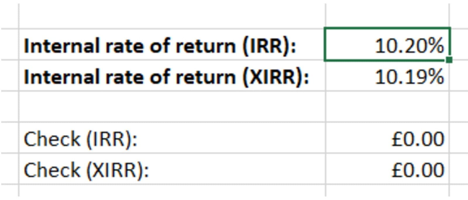
Because IRR’s calculation method matches NPV, and XIRR’s matches XNPV, you can use the corresponding functions to check that the results are indeed £0:

Because these aren’t precise calculations, if you expand out the decimals, eventually you’ll see a few nonzero amounts, but this is nothing to worry about.

It’s very important to remember the difference between these two functions and how they calculate – NPV and IRR start discounting immediately, whereas XNPV and XIRR discount later cash flows back to the first one listed. If you forget this you can easily end up a year out on your discounting!

Check out the accompanying example file and experiment with the functions for yourself.

You may also like

• Previous post - Workbook viewing redux
• TOTW index
• Next post – The limits of Excel