Hello all and welcome back to the Excel Tip of the Week! This week, we have a Creator level post in which we are looking at how to use Power Query to generate a couple of common kinds of transaction reference easily and automatically – including one that’s incredibly hard to do with just formulas alone.
Transaction numbers by customer
First, we will look at a situation such as this:
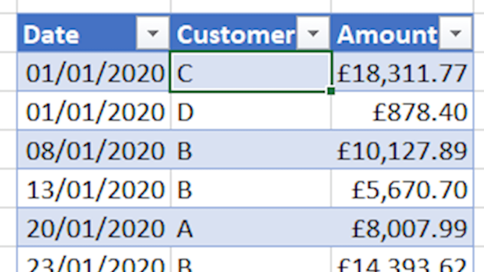
Here we have invoices for a selection of customers, and want to assign each a sequential number based on the customer. Of course this approach also works for numbering within each date, or via some other field – we’re just using customer name as an example.
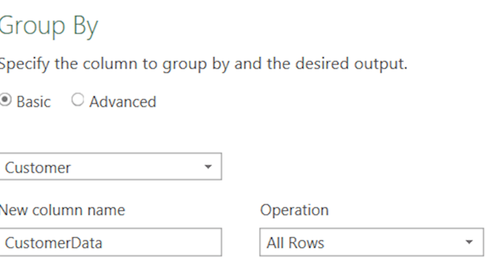
We start by loading our data into Power Query with Data => From Table/Range. This will let us work with the data. Our first step is to group the table by the Customer column, selecting ‘All Rows’ as our grouping type:

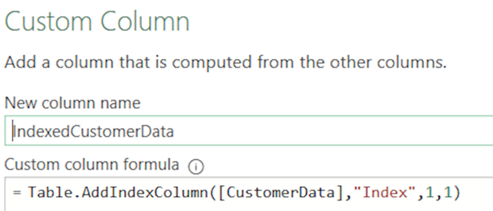
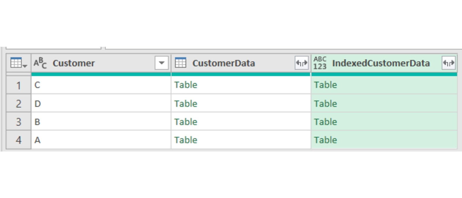
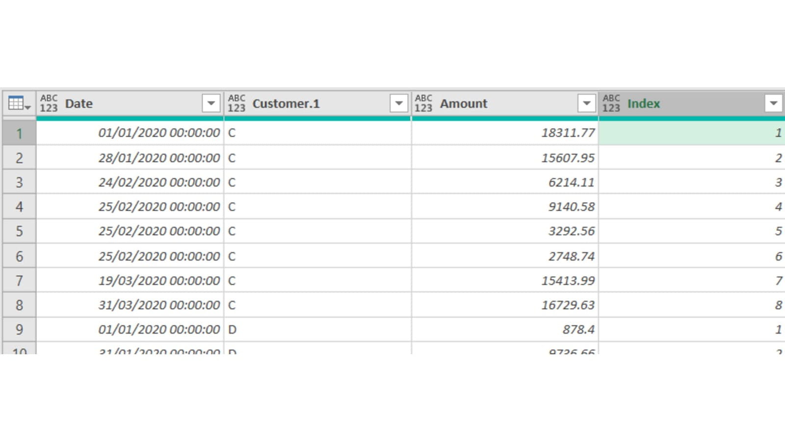
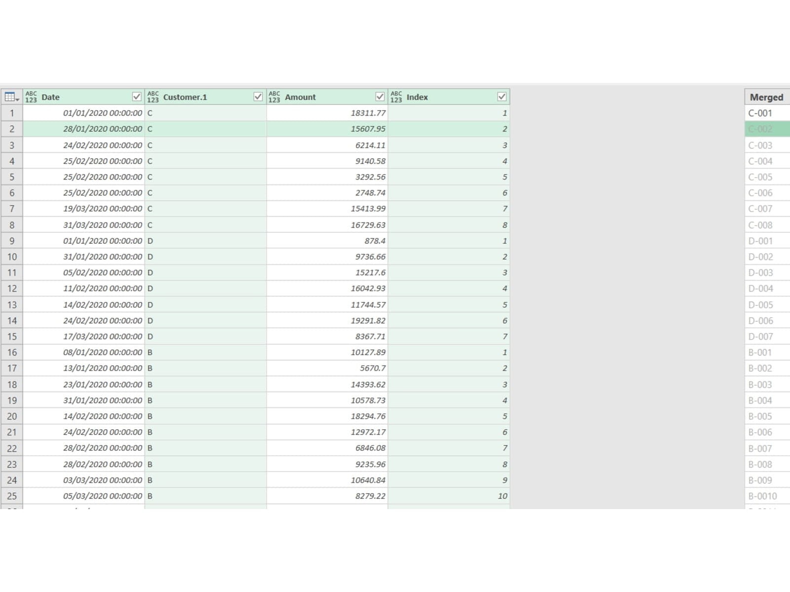
Here we just write the first number and Excel’s AI does its best to predict the rest. We can see that the 10th B invoice is “B-0010” rather than “B-010”, but if we correct that one manually Excel will correctly figure out what we want, which is this M code:
=Table.AddColumn(#"Removed Columns", "Custom", each Text.Combine({[Customer.1], "-", Text.PadStart(Text.From([Index], "en-GB"), 3, "0")}), type text)
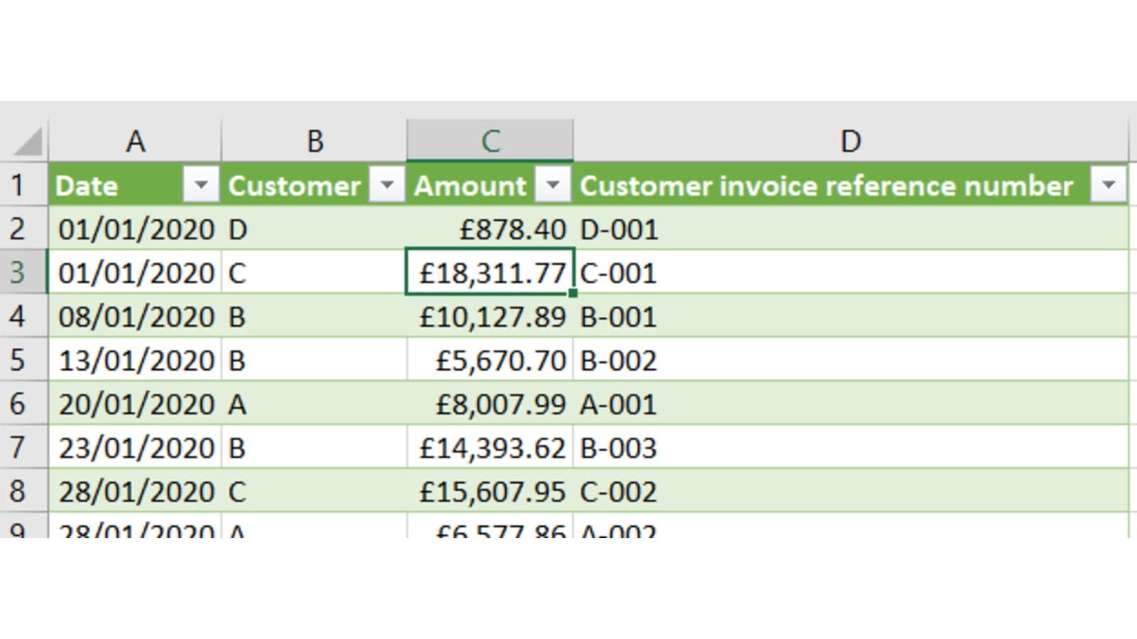
Then we can just tidy up our column names, remove duplicates, and export:
Creating references from a summary
The above example is possible with Excel formulas, but now we are going to look at something that is beyond what’s practical with formulas alone – creating a full numbered listing from a summary.
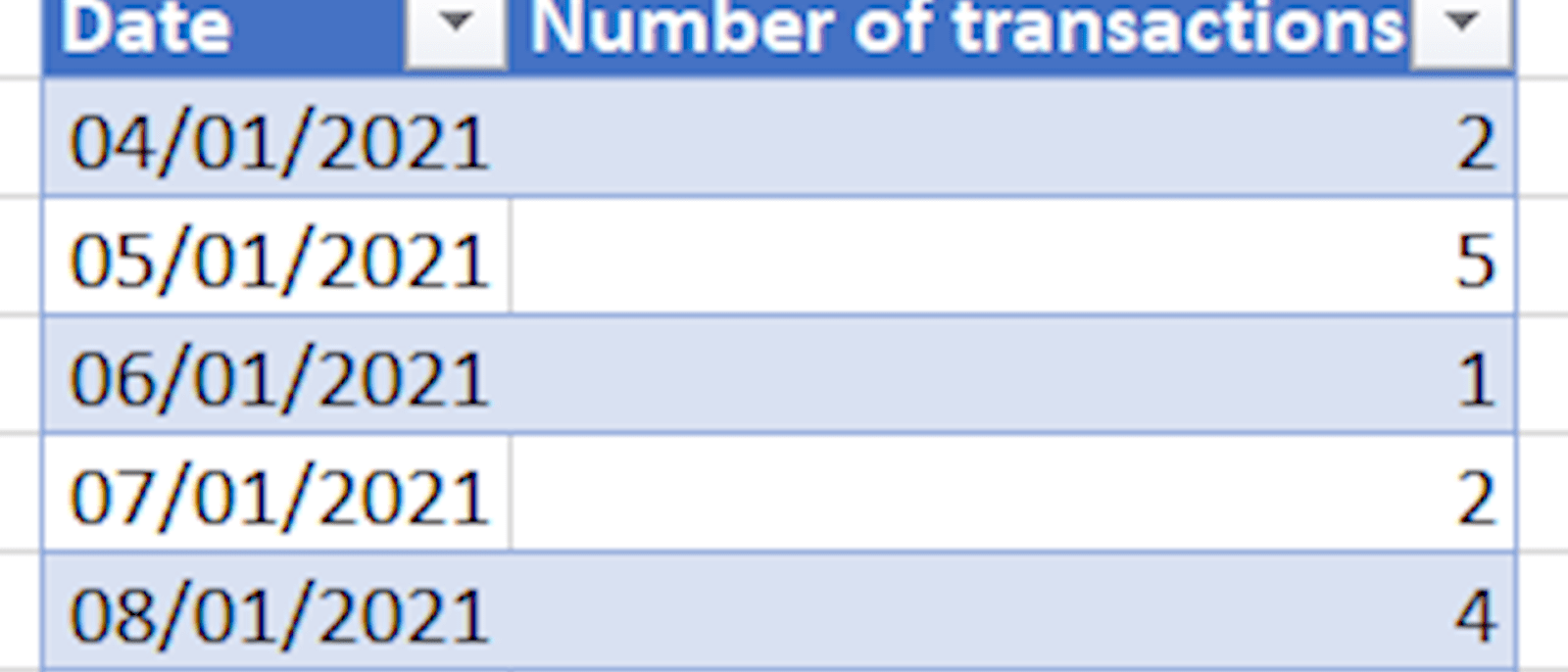
Here’s the data we’re working with this time:
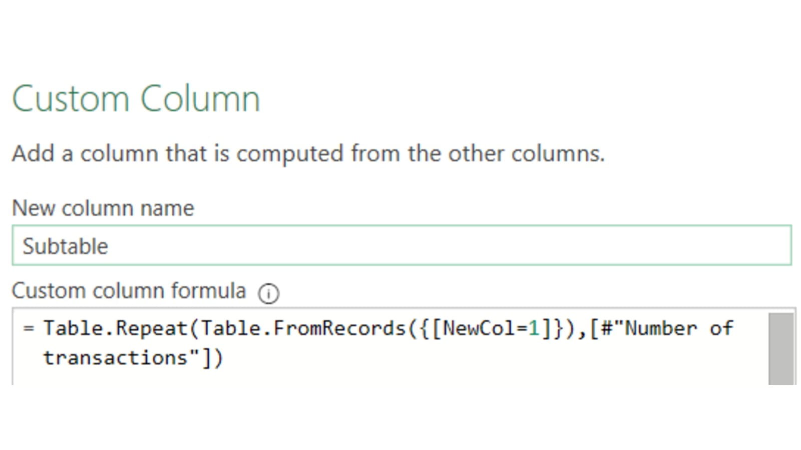
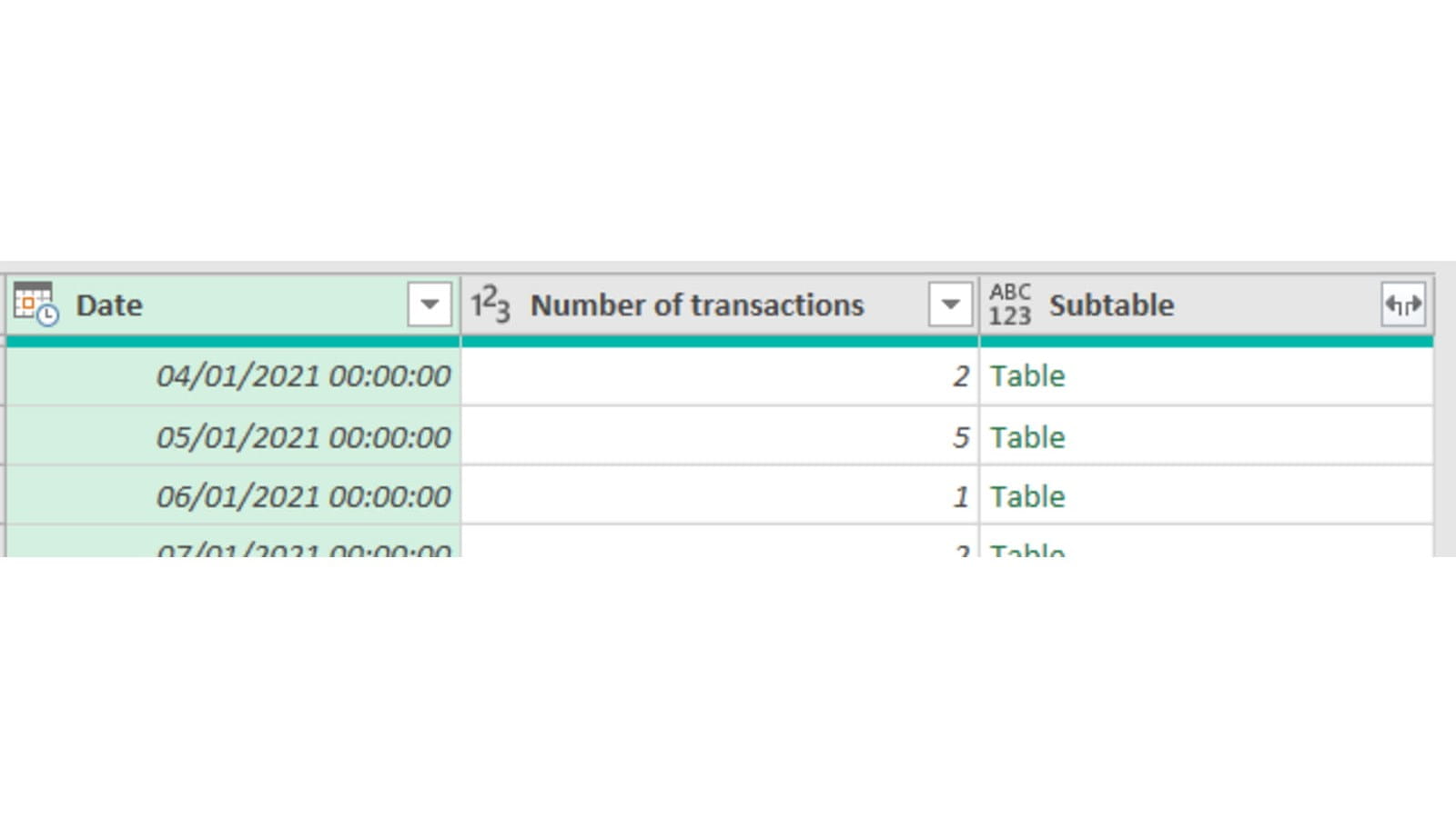
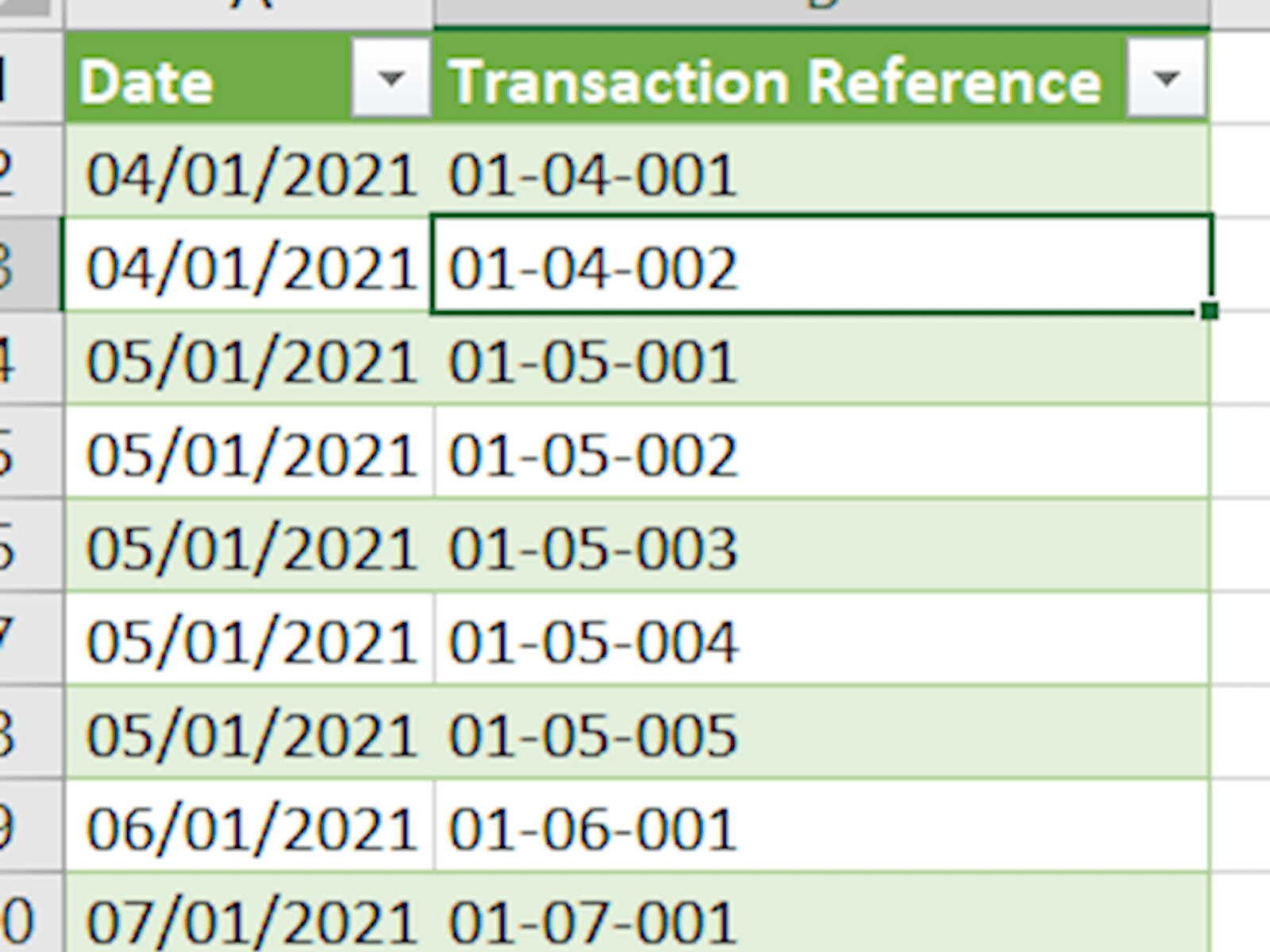
You can see both sets of data, both queries, and the final results in this file
You may also like
Excel community
This article is brought to you by the Excel Community where you can find additional extended articles and webinar recordings on a variety of Excel related topics. In addition to live training events, Excel Community members have access to a full suite of online training modules from Excel with Business.

Archive and Knowledge Base
This archive of Excel Community content from the ION platform will allow you to read the content of the articles but the functionality on the pages is limited. The ION search box, tags and navigation buttons on the archived pages will not work. Pages will load more slowly than a live website. You may be able to follow links to other articles but if this does not work, please return to the archive search. You can also search our Knowledge Base for access to all articles, new and archived, organised by topic.

