Hello all and welcome back to Excel Tips and Tricks! This week we’re digging in the archives to return to a topic familiar to many, but with some additional secret Windows functionality that’s worth highlighting.

In this Basic User post we're going to explain the various ways to create an image of an Excel spreadsheet, or just part of it. Whether you need a capture for a presentation, or to create documentation, or to make an illustration for a popular weekly Excel tip series, screenshotting is a natural part of the Excel workflow. But you might not know that there are some handy options available to make your life easier!

Print Screen

Windows supports a simple print screen function, which most keyboards and laptops dedicate a button to (or double up with a function key). In case you aren't familiar, this button will put a copy of what's on your screen into your clipboard. From there, you can paste to get a copy of the image wherever you're working.

Pros: Simple, quick

Cons: Can only capture the full screen at once, unless…

Print Screen shortcut (new feature!)

There’s a little-known Windows setting that opens up more functionality to the Print Screen button. 

If you go to your Windows Settings (press Start and type ‘Settings’) and go to Ease of Access > Keyboard, buried near the bottom of the page is the setting for ‘Print Screen shortcut’

If this is turned On, when you next hit the Print Screen button, instead of automatically taking a snapshot of the full screen, you’ll be presented with the ‘Snip & Sketch’ options:

These allow you to:

• select a rectangular region of the screen
• select a freeform region of the screen
• select a currently active window
• select the entire screen.

Once actioned, your screenshot is saved to the clipboard to be pasted into your document. However, if you click on the notification, you can open the Snip & Sketch tool to further annotate, crop, save and share your screenshot (as well as copy to the clipboard):

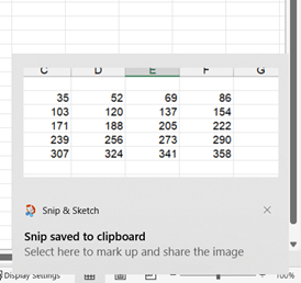
Snip & Sketch can also be accessed from the Start menu where you have the additional option of adding a 3 or 10 second delay before taking the screenshot, in case you need that ‘action’ shot to be just so.

Pros: Specific capture, ability to annotate

Cons: Can only clip active windows

Insert Screenshot

This option, found on the Insert Ribbon under Illustrations in Excel, can quickly create and post an image of any other window that you have open, and instantly paste it into the current workbook:

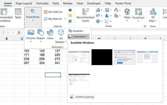
You can also use the 'Screen Clipping' tool at the bottom to instead draw a box and capture just part of one of the other windows.

Pros: Specific capture, quick

Cons: Can't capture from within the active workbook (but as a workaround, you can use the same functionality in Word or PowerPoint to capture an Excel workbook)

Paste as picture

If you just want to capture the contents of some cells, you can copy those cells and then paste as an image:

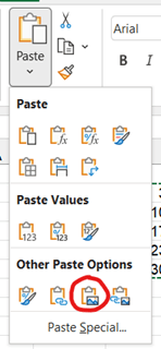
Note that this option is not on the standard Paste Special menu!

Pasting will create a static image of your cells. It's transparent, which can make seeing it against an Excel backdrop a bit difficult, but it's an exact crop of what you copied so is useful for getting an accurate snapshot into another program.

Pros: Cell-exact capture

Cons: Harder to access, can be hard to read

Paste as linked picture

On the same menu as Paste as Image (on the Home Ribbon, right click menu or if you press Ctrl after doing Ctrl+V), there's an option to paste as a linked image just to the right:

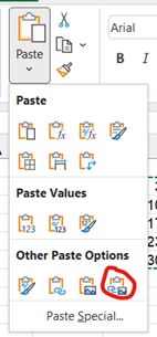
This has a similar appearance to the before - but with one key difference. This linked picture is linked to the live cells - so if you make a change to the cells, the picture is changed also. You can see that when you select the picture, a sort of formula is shown in the formula bar; indeed, you can change this formula to edit what is shown in the picture:

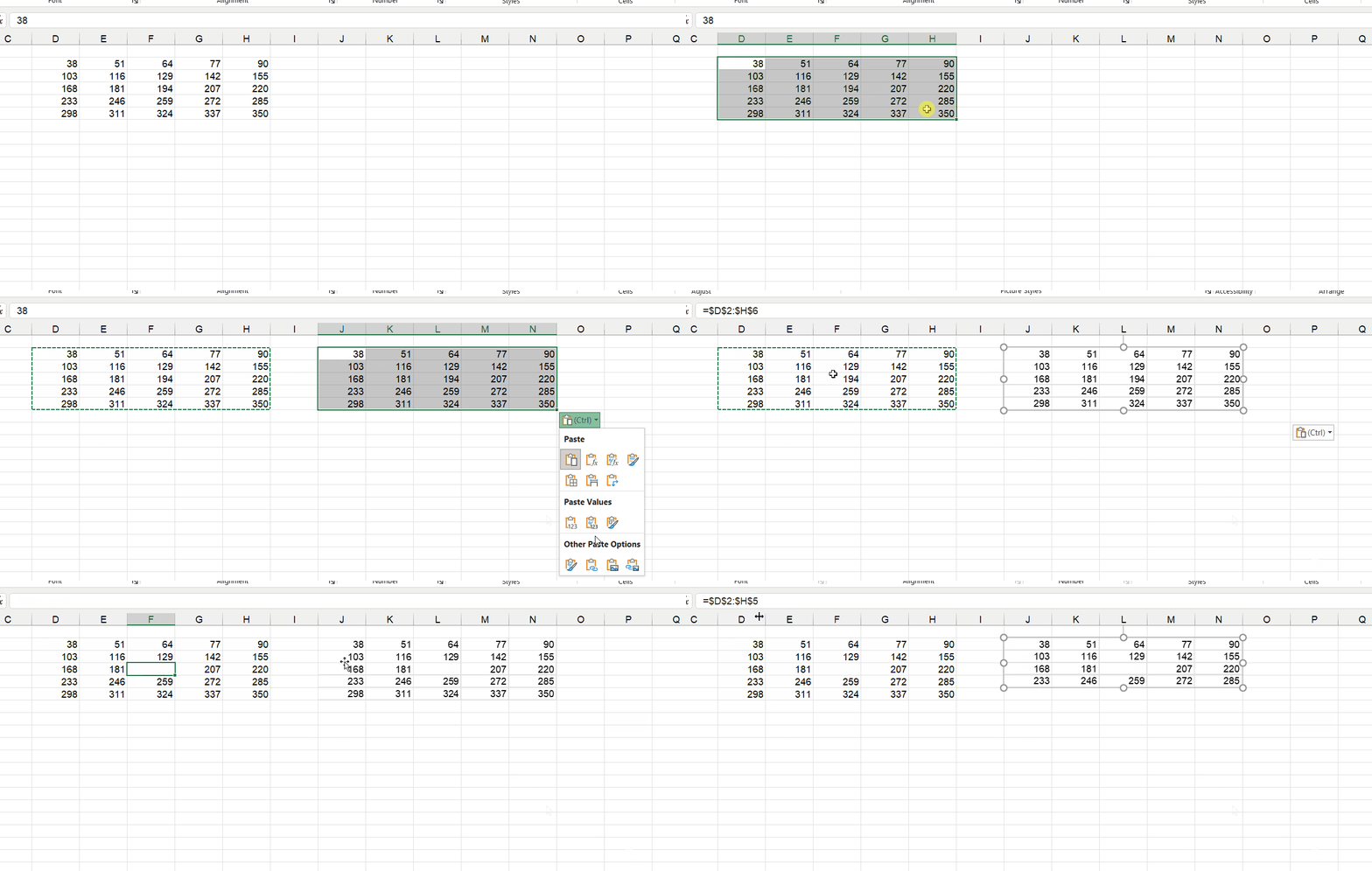
Unfortunately, the link lasts only as long as the picture remains in Excel - copy it into another program, and it will become just a static image.

Pros: Live updating, easy editability

Cons: Harder to access, doesn't work outside of Excel

And that's the guide!