Excel Tips and Tricks #445 – Filter/Sheet Views

Why Filters are Annoying

In the past (or, in some cases, still the present), collaborating on spreadsheets generally meant either sending them back and forth by email, or putting them on a network drive where if more than one person tried to open the file, you’d get this wonderful message:

However, crucially, because you couldn’t have two people editing a spreadsheet at the same time, you never got into trouble where one person did something to the spreadsheet that messed up what the other person was working on.

And then, along came Google Sheets.

People would now be able to actually see other people, in the spreadsheet, at the same time. Different people could edit the document simultaneously. It was joyous.

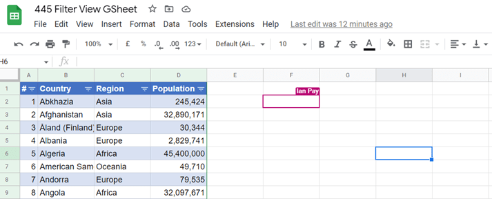
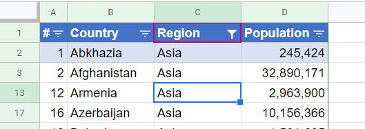
It was also infuriating. Because if one person applied a filter, that filter would be applied for everyone at the same time. Oi, I was working on row 10!

Even worse was if some people only had read access; the editor might apply a filter and then those viewing the spreadsheet would be snookered – unable to remove the filter, unable to view the data they wanted to see.

Google developed functionality to accommodate different ‘views’ of the spreadsheet – people could be looking at the same sheet, but be seeing different filters on the data at the same time. It is functionality that for several years was absent from Excel but has recently been introduced.

It’s a bit hidden away, and not very well explained within the applications, so let’s deal with that now.

Principles of Spreadsheet Views

‘Views’ in both Excel and Google Sheets are basically the same – that different users can look at a sheet in different ways, at the same time, without impacting the work of each other.

There are two main aspects of these views:

• Saved views
• Temporary views

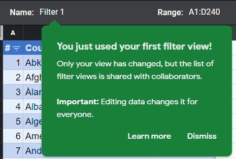
Saved views can be created by anyone with edit access to a spreadsheet and can be used to store a particular set of filters for quick access – in my countries spreadsheet from Tip #443, I might have different views for each region, for example. Or, if working with a small team, you can give members of the team their own designated view so that they can work with the sheet however they want to without filtering out content that other users were interacting with.

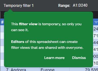
Temporary views, meanwhile, are just that – they only exist while being used, for the user who created them, and cannot be saved for future use.

Don’t forget – data can still be edited in views (if you have the permissions to do so), and those edits affect everyone. So just because you are in a filter or sheet view doesn’t mean the changes you make to cell contents won’t be seen by others!

A feature that is consistent with both Google Sheets and Excel is that when you are in a view, the row/column headings turn dark, to make it easier to tell when you are in a user-specific view, compared to the default view.

(NB 1 – if you use a ‘dark’ Office Theme, the colour change is barely distinguishable so watch out!)

(NB 2 – if your Excel settings have the headings hidden (View>Show>Headings), you won’t see this at all – look out for the microscopic eye on the tab at the bottom of the screen!)

The way that Google Sheets and Excel deploy views is slightly different, so we’ll just spend a few moments discussing each in turn.

Google Sheets – “Filter Views”

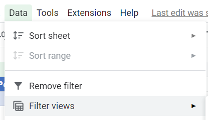
Filter Views are accessible from the ‘Data’ menu:

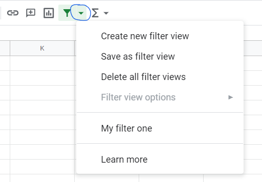
Or can be accessed with the drop-down arrow for filters on the toolbar, which gives the same menu:

The first set of options are fairly self-explanatory. When you have saved filter views, you can select them on this menu. Saved filter views are available to all users of the sheet, but only editors can change them – this includes changing the filters within them.

Filter view options allow an editor to rename, duplicate, delete or update the range for a saved view (see below for the implications of this last one).

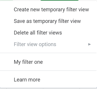
If you only have view access to a Google Sheet, you’ll have slightly different options:

These work in a similar way, but the views are only created and saved temporarily; if you close and reopen, or refresh, the sheet, the temporary views will disappear. The saved views are available to use, but viewers cannot change the filters in them.

(At the time of writing, ‘Delete all filter views’ has a bug that means viewers can appear to delete all filter views, but in fact only delete them in their current session; refreshing the page restores any saved filter views)

Crucially, the clue is in the title - Filter Views are based around filters. In practice, this means the view (saved or temporary) includes the range definition that the filter is applied to – which may require manual updating if your data set changes in size – and the view only really impacts the filter and nothing else about the sheet such as hidden rows/columns or cell sizes.

One feature of Filter Views to note is that when you have a filter view open, you can copy the URL to provide other users with a direct link to the file with the filter view applied.

Excel – “Sheet View”

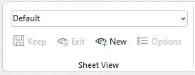
Sheet View is accessible from the ‘View’ tab in both desktop and web versions of Excel 365.

At a basic level, for editors, Sheet View is similar to the Filter Views in Google Sheets. You can create a new view, save it, manage and switch between saved views, and go back to the default view.

If you only have view access to the Excel file, it all works a little differently – you won’t have access to the ‘Sheet View’ functionality as, in effect, your entire experience of the workbook is as a temporary view. This means you can filter and sort the data without touching the saved version.

In Excel, views apply to the whole sheet, not just the filter. This means a couple of important differences compared to Google Sheets:

• Any filter on the data set is defined separately to the view – this means that you cannot have different views filtering on different ranges of data (in Google Sheets, you can). If there is no filter set up on the dataset, a user with only view access will not be able to add one.
• On the flip side, in sheet views users can make other changes to the display of the sheet, such as showing and hiding rows, and changing row/column heights/widths, and these changes are not reflected in the default view (something that you cannot do in Google Sheets). However, such changes are also only temporary, so as soon as the view is closed, cell sizes and show/hide settings revert to the default view.

Your Own View on the World

The joy of views, in both Google Sheets and Excel, is that you can explore the data on the sheet to your heart’s content, without it having any impact on other users. It is a vital part of the collaboration features in both applications, and if used properly, never again will you have to shout to your colleagues “can you take the filter off the spreadsheet please, I was working in row 10!”