• View the webinar recording here

How do you set up so that when you go to print the maximum page space is printed?

First of all, I recommend trying to avoid printing Excel files wherever you can. The program just isn’t very print-friendly and losing the ability to check formulas is a big downside.

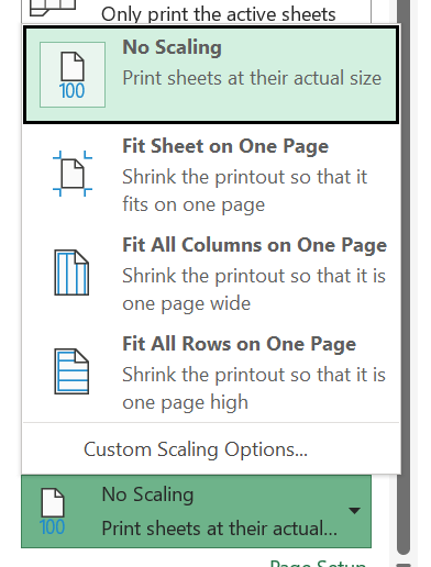
That being said, there are a few general tips for maximising print effectiveness. First of all, use View => Print preview to get an idea of where the different elements of your spreadsheet would be printed according to your current settings. Try using landscape orientation and rearranging your data to get the best fit. And then when printing, the scaling dialogue is very useful for getting your file to fit as closely to the page as possible:

SORT function - I find this really useful but is there a way to use it (or a similar function) to sort multiple columns in a data range?

You can use SORTBY to do this:

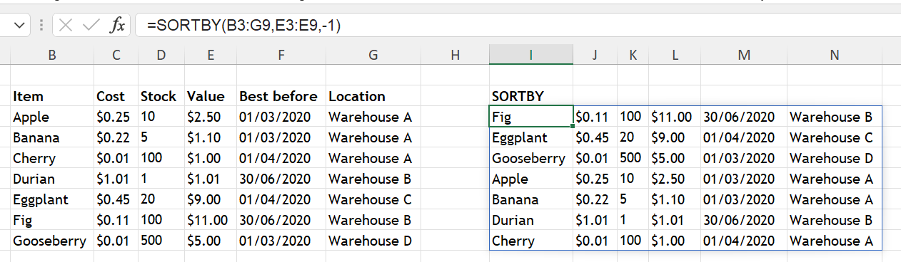
The general idea is:

=SORTBY(range to sort, column to sort by, +1 for ascending or -1 for descending)

Is there any way around not being able to copy multiple tabs that contain tables?

Unfortunately not. If need be you can convert tables back to standard cells from the special Table => Manage menu.

I often have difficulty with understanding H and VLOOKUPs, where I'm not sure if it's the data I'm looking at that needs to be sorted first, or the query data.

These formulas don’t require the data to be sorted, but you must specify that you only want to return exact matches by including FALSE or 0 as the fourth argument in the formula. Otherwise they won’t work.

Note that the newer XLOOKUP function can replace both of these and doesn’t require specifying, so if you have that then it’s the better option.

Is there an Excel NPV calculation that works according to dates rather than a period?

Related to the NPV question; I remember being warned off NPV function for a few reasons including the period point. Does XNPV solve all these problems or are there still issues with it?

Yes, XNPV:

=XNPV(rate, values, date)

The main thing to remember is that XNPV discounts the cash flows to the date of the first one specified, so if you want to know the value at another date then further calculation will be needed.

Can you explain a scenario for which you could use the SUMIF tool please?

SUMIF or its more flexible cousin SUMIFS can be used any time you want to add up numbers that meet certain conditions. For example add up only the positive values in a column:

=SUMIFS(column, column, “>0”)

Or add up the invoices that match a certain name written in A1:

=SUMIFS(invoice amount column, name column, A1)

I have a list of various dates in format 25/01/2022 but I'm only interested in knowing the month (or perhaps the year) but unsure what I need to do efficiently?

You can use the MONTH and YEAR functions to extract them into different cells.

Can you explain the INDIRECT function and when it can be used please?

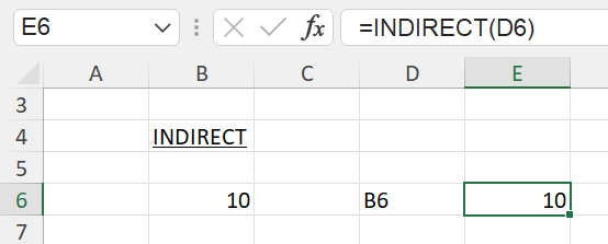
INDIRECT will look at its input and try to interpret it as a cell reference. If it can do that then it will return the value found at that reference:

For pivot tables, there is an option to generate a tab for each filter item - can you go through how we do this and how the pivot should be set up?

This can be done for a Pivot with a filter applied to it. There is one prerequisite though – you need to uncheck “Add this data to the Data Model” when inserting the PivotTable.

Once you’ve done that, set up your Pivot and then go to PivotTable Analyze => Options => Show Report Filter Pages. This will quickly create a copy of the PivotTable for each option in the filter.

Can you give a quick overview of ways of reviewing data - duplicates, statistical outliers etc please?

There are lots of aspects to this question, and for a more in-depth answer I recommend checking out our free guide How to review a spreadsheet.

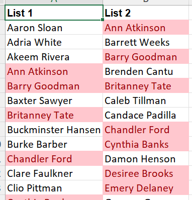
For some basics, you can start by detecting duplicates with Home => Conditional Formatting => Highlight Cells Rules => Duplicate Values. This is very good for quick comparisons between two lists:

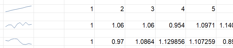
For spotting outliers or other unusual values, there are plenty of statistical functions in Excel to help you here, but for a quick start I like using a chart or sparklines to check visually for anything that looks unusual.

How did you add the $ signs quickly to the formula when you were demonstrating the XLOOKUP?

There’s a keyboard shortcut – press F4 while entering a range will toggle the absolute/relative referencing settings by cycling through where the $s could be added.

I’d value some general tips on dealing with large data sheets: moving around the sheet quickly, highlighting blocks of data, sorting, filtering, cutting filtered items from a master sheet on to another sheet etc.

You can quickly navigate by holding Ctrl while pressing the arrow keys to jump over blocks of empty or filled cells. Hold Shift as well to select the cells as you pass through them.

Sorting and filtering are best done with Data => Filter. You can cut and paste from a filtered range just fine, but if it isn’t working quite right, try using Alt ; to reduce your selection to only the currently visible cells.

Do the “Principles” tell us what steps to follow when creating a worksheet from scratch? Eg a quick Google of existing templates (any recommended web sites?), or perhaps a 1,2,3 of steps to follow?

The 20 Principles document is more high-level than that, but templates are a good start if you’re doing something specific. We are currently working on collating all the ones that the Excel Community has produced, so look out for that in the future!

Can INDIRECT be used with the SORT or FILTER functions?

In theory yes, although I can’t immediately think of a use.

How do I set up a report so that I can link it to a table on another sheet and easily select column I display? eg Q1, Q2 etc.  Do I need to use named ranges?

I would suggest basing your report on an Excel Table (added with Ctrl T or from the Home menu), potentially creating a PivotTable depending on your exact parameters, and then using a Slicer to control what data is shown.

Are there any particular recommendations you have for the Quick Access Toolbar?

Just to provide some background to this question – the Quick Access Toolbar is the very top left of the Excel window, where some buttons for very common tasks like saving are kept:

You can use the Options menu to customise this, adding or removing things you use particularly often. I’m not a big user of it – I prefer keyboard shortcuts – but a lot of people like it for e.g. pasting values.

Can you take us through the OFFSET formula please?

OFFSET is a formula that takes as its inputs a single cell address and two numbers. It moves (offsets) that many rows & columns from the starting cell and returns the value of the cell it lands on. It looks like this:

=OFFSET(starting cell, row number, column number)

It’s often used to make things like scenario pickers, although I much prefer INDEX for that.

You can also add a height and weight as two further inputs to have OFFSET draw a range starting at the landing cell. If you’re doing that you would normally put the whole OFFSET inside another function that can do something with that range – e.g.:

=SUM(OFFSET(starting cell, row number, column number, height, width))

Is there an easy way to change the format of negative numbers from "-1" to "(1)”?

Can you set this format as the default?

I went into quite a lot of detail during the live recording about how custom Excel formats work – see TOTW #332 for a primer on those. The basic number format to use for negative numbers is something like:

#,##0_);(#,##0)

If you want to reuse this format frequently without making it manually, then you can do this by customising a cell style – see TOTW #251 for an in-depth explanation.

Is there an alternative to nested IF statements please?

Yes, depending on what you’re trying to do with your nested IFs! It might be better to use a lookup function, an IFS or SWITCH, or something else entirely – feel free to contact us at excel@icaew.com for more specific ideas.

When trying to use the MATCH function recently, I encountered a floating point issue that prevented it working. I ended up with a ridiculously complicated formula to get round the problem. Are there any other common Excel formulae that are particularly vulnerable to floating point errors?

Floating point errors are tiny rounding differences that arise in Excel when it converts between the decimal numbers that we use to the binary numbers that computers use. While there are a lot of automatic error-catching features in Excel that try to prevent them, no computer system is 100% foolproof and so sometimes calculations can return results like 20.0000000001 that are very slightly off from expected.

These aren’t an issue for further mathematical functions like SUM, as the differences are so tiny. But they can be an issue for anything that’s looking for an exact match – like a MATCH or other lookup function. Using a rounding function on the formulas that are throwing up floating point errors will fix this most of the time.

When using XLOOKUP, can you use it on data that is in horizontal?

Yes, it works on both and so effectively replaces both VLOOKUP and HLOOKUP.

Is there a way to turn sparklines upside down ie data is all credits and you want most negative to be shown as higher?

Sparklines (discussed in TOTW #290) are tiny one-cell charts that can be used for a quick overview of your data:

They are very simple with few options, so they can’t do what you want here; you would need to create a (possibly hidden) formula row that inverted the values with formulas and then chart that instead.

What's the benefit of formatting your data as a table?

An Excel Table, added from the Home menu or with Ctrl T, adds an XML object to your sheet that contains your data:

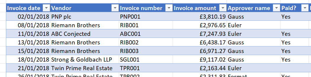
This has several advantages:

• Tables automatically expand when new data is added next to them, making formatting consistency easier
• The filter handles at the top of Tables remain visible even when the actual header row is scrolled off the top of the sheet
• Tables automatically copy formulas to the entire column
• You can assign names to Tables, and then use those names in formulas to make easy dynamic references; e.g. =SUM(TableName[Column name])

May I know whether I can highlight the specific words in the cell (not the whole cell)?

This is called rich formatting – Excel supports it but only to an extent. You can add a format like a font colour or underline to just part of a cell, but not a highlight. You also can’t do this with VBA or conditional formatting, only manually.

Is there a way to import TB in a tabular format directly from Xero using the get Data function please?

I am not familiar with Xero, but it’s at least possible with Power BI which uses the same backend as Power Query, so it may well be doable!