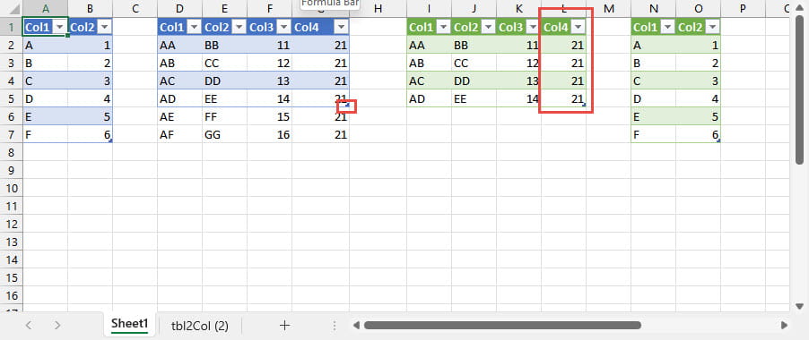
Here we have some dummy Tables. Rather than adding and removing data, we will use the Table marker in the bottom right-hand corner of each source Table (in blue) to change the number of rows and then columns in use:

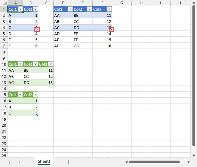
If we increase the number of rows in our 3-column source Table, and Refresh our green output Tables, we can see that the top Table expands downwards and automatically moves the 2 column Table beneath down to allow room:

However, if we reverse the position of our Two Tables and then increase the number of rows in use in our 2-column Table, we will see that things don't go as well:

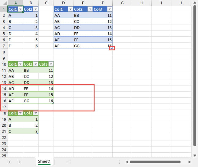
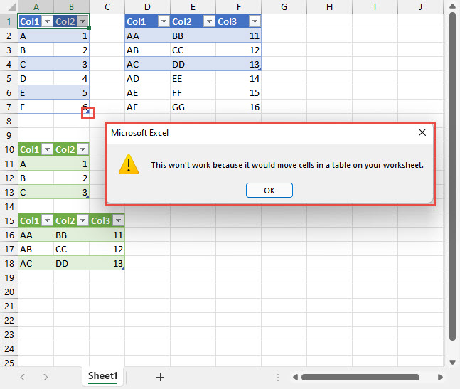
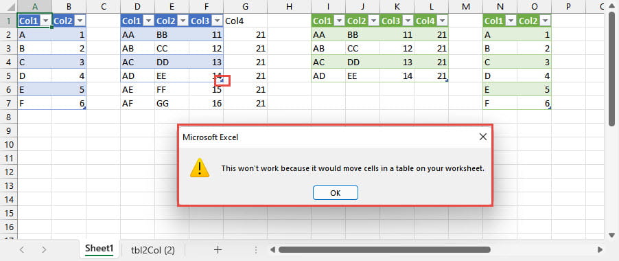
The problem is that, with fewer columns in the top Table, not all the rows in our green 3-column Table are moved, hence the message that the refresh fails because cells would be moved within a Table, rather than the entire Table being displaced. This would also be a problem if the number of rows in the source Table was reduced rather than increased.

We can avoid the issue by changing the Table Properties. Here we have right-clicked in our 2-column Table, chosen Table, External Data Properties… and then selected the second of the options in the section:

Data formatting and layout, If the number of rows in the data range changes upon refresh:

As the description of this option suggests, rather than just inserting cells, this option caused the Table to insert whole rows as it expands, ensuring that it moves the entire Table below, even if it has more columns:

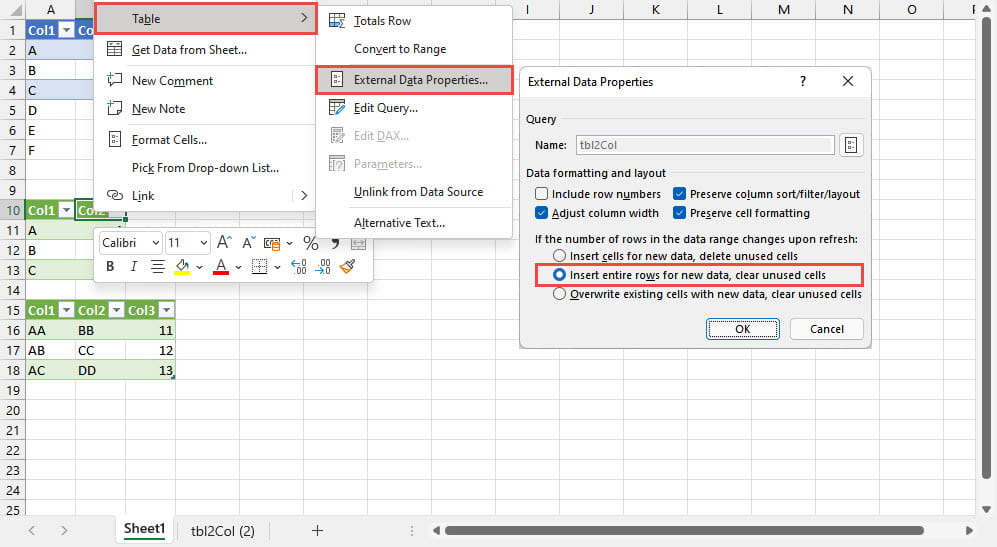
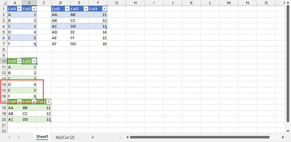
As you can see from the above screenshot, this is not perfect as it causes our 2-column Table to overwrite the blank cells separating our two tables as well as moving our 3-column Table down, but at least it does allow the Tables to refresh successfully.

There are similar problems if we arrange our Tables horizontally rather than vertically and we change the number of columns in the source Table. Tables to the right can be moved when the number of columns increases:

However, if we then reduce the number of columns in our left-hand Table our error message appears again:

In summary, if you do try and combine refreshable Tables in a single worksheet you do need to think very carefully about what will happen should the number of rows and/or columns change. Generally, the number of columns is likely to be more predictable so you could try and ensure your Tables all have the same number of columns, even if it means padding some of the Tables with empty columns. Otherwise, if the number of rows might vary, you will need to arrange the Tables so that Tables with more columns are positioned above those with fewer columns.

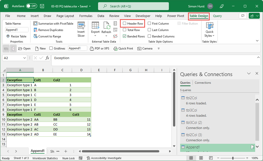
There are also some more creative solutions available to deal with the problem. Here, we have used Power Query to add a description column to each of our Tables, set the option in the Home Ribbon tab, Transform group to 'Use Headers as First Row' then Appended our Tables to create a single Table that includes all our exceptions. In the resulting Excel Table, we have turned off the display of the Header Row in the Table Design Ribbon Tab, Table Style Options group, and used Conditional Formatting to set the font of our heading rows to Bold and with a darker fill colour: