Animated Excel Christmas tree

Introduction

Inspired by the idea of Excel Pixel Art mentioned in a recent article, I thought I’d try and create an animated Christmas card in an Excel worksheet. I decided to keep things relatively simple and go for a Christmas tree with coloured lights.

I started off creating a ‘normal’ formula that needed to be copied to all the cells where the Christmas tree might appear, and then moved on to seeing if I could use a Dynamic Array to create a Christmas tree using a single formula. The solution I came up with involved the use of the MAKEARRAY() function which uses a LAMBDA() function as one of its arguments. I can’t help thinking that there’s probably a vastly simpler way of achieving what I was aiming for, so if you run out of productive things to do at some point over the Christmas break you could always try and find a better solution:

Conditional formatting

We have changed the column width and row heights for the tree area to create small squares, each of which can hold a value and be formatted with a colour. Worksheet gridlines have also been turned off.

The workbook uses conditional formatting to format the fill and font colour of individual cells depending on their position to ensure that any cell contents are not visible. The formula just draws the triangle part of the tree, with conditional formatting coping with the trunk on its own.

For a bit of interactivity, we have added Scroll Bars to control the size of the tree and the number of lights.

It is possible to cover the entire tree in lights, but generally we will want more green tree than multicoloured lights. We achieve this by generating a random number between a minimum and maximum value and then formatting a proportion of the possible values to be green, while the remainder are set to one of 5 other colours:

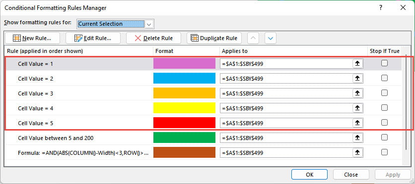
Values of 1 to 5 are formatted in the five colours, with values over 5 and below 200 being Christmas tree green. This means that, the higher we set the maximum value for the RANDBETWEEN() element of our formula, the lower the proportion of lights to tree.

Our final conditional format is used to colour the trunk cells and we’ll look at this in more detail shortly.

Static formula

Before we look at the Dynamic Array solution, we will just use a formula that will need to be copied to all the relevant cells:

=IF(AND(ROW()<Width,COLUMN()>Width-(ROW()-1),COLUMN()<Width+(ROW()-1)),RANDBETWEEN(1,Lights),"")

In order to draw our Christmas tree shape, we use the ROW() and COLUMN() functions to work out whether we need to allocate a number to each cell or to leave it blank. Where we need a number, we use the RANDBETWEEN() function to add a number between 1 and a maximum determined by the value in the cell to which we have allocated the Range Name ‘Lights’. The formula in the ‘Lights’ cell subtracts the value in a different cell. that is linked to our Lights: Scroll Bar, from a pre-set maximum. So, as we drag the scroll bar to increase its value, the maximum value will decrease, increasing the proportion of lights to tree.

Our IF() function checks three conditions:

ROW()<Width

Firstly, the cell must be in a row that is less than our ‘width’ value. The tree section will have two rows fewer than the width value and twice as many columns. To give our Christmas tree shape, the tree needs to get wider as we go down the rows, so the next two conditions add columns to the left and right of our centre point respectively, increasing according to the increasing row numbers:

COLUMN()>Width-(ROW()-1),COLUMN()<Width+(ROW()-1)

The only reason for subtracting 1 from the ROW() value is to cope with having used row 1 for our two scroll bars. The two conditions check which columns in each row should be allocated numbers. As we go down the rows, the number of columns will increase by one to the right and one to the left of the central position as the ROW() number increases by one.

The full formula needs to be copied to our large block of formatted cells and we apply our conditional format to the same cells. This creates our tree area. The trunk just uses conditional formatting:

=AND(ABS(COLUMN()-Width)<3,ROW()>=Width,ROW()<Width*2)

Our conditional format formula will return TRUE for cells in columns less than three columns to the left or right of the central position. The ABS() function treats positive and negative numbers as being positive so allows for column numbers less than, as well as more than, our central column number. The conditional format also starts our trunk at the bottom of the tree – from the Width value downwards and extends to the same length as the Width value.

The Scroll Bars

The Developer Ribbon tab, Controls group, Insert dropdown includes a Scroll Bar form control. We can ‘draw’ our control onto our worksheet and then right click on it and choose Format Control to set our Scroll Bar settings, including allocated the result to a cell to which we have given an appropriate Range Name:

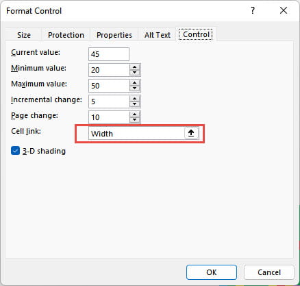
By dragging our Tree size bar to the right, we will increase the size of the tree. By dragging our Lights scroll bar to the right we will increase the proportion of lights up to having the tree completely hidden in lights.

Dynamic Array

In essence, we just convert the formula that we have just been looking at to a LAMBDA() function:

=LAMBDA(treerow,treecolumn,IF(AND(treerow<Width,treecolumn>Width-treerow,treecolumn<Width+treerow),RANDBETWEEN(1,Lights),""))

Our one formula has to cope with all the rows and columns to which we copy it, so we convert our uses of ROW() and COLUMN() to the parameters: treerow and treecolumn. When we use our LAMBDA() function we pass the appropriate row and column numbers to these two LAMBDA() parameters. We do this as part of the MAKEARRAY() function. This function takes a number of rows and a number of columns as its first two arguments to determine how big the array will be. The third argument is our LAMBDA() function. You might be wondering where the treerow and treecolumn values are entered. MAKEARRAY() passes the row and column indices of each cell in the array as values to our LAMBDA() function, which is exactly what we want to do, so we don’t need to explicitly specify these values:

=MAKEARRAY(Width-1,(Width-1)*2,LAMBDA(treerow,treecolumn,IF(AND(treerow<Width,treecolumn>Width-treerow,treecolumn<Width+treerow),RANDBETWEEN(1,Lights),"")))

Wherever you enter the formula, as long as there are enough empty cells, Excel will draw your Christmas tree according to the Width and Lights values set by the Scroll Bars, though you will need to set up the conditional formatting to add the colours and the trunk.

The ever-changing lights

Because of the use of RANDBETWEEN(), the position and colour of the lights should change whenever the spreadsheet is recalculated. You can trigger a recalculation manually by pressing the F9 key to ‘Calculate Now’ or use the equivalent command in the Calculation group of the Formulas Ribbon tab.

Conclusion

If you really do end up with too much spare time over Christmas, you could always try and add an appropriate pot or stand for your Christmas tree and make the height and width of the trunk changeable based on cell values. Perhaps adding a coloured background with random snowflakes might be going a bit too far.

You can explore any of the various techniques we have covered here in the ICAEW Excel Community archive.