Organisation Data Types

Excel Data Types have had rather a difficult history. Originally, Microsoft had intended that the feature would include an extensive range of different Data Type, most made available through Microsoft’s collaboration with Wolfram Alpha. However, apart from a few fleeting glimpses of the full list of data type in Excel updates that were quickly followed by another update removing them again, they never made it to general release, in the UK at least. Then, about a year ago, Microsoft announced that their partnership with Wolfram Alpha to support the Data Types would not be renewed, with the ability to create new Data Types, or refresh existing ones in Excel, ending on June 11th 2023.

Although the Wolfram Alpha Data Types are no longer available, there are two ways to create your own Data Types. Power Query includes an option to create Tables with Structured Columns that behave in a similar way to the use of a Data Table. The other option is the use of the Organisation Data Type to include Data Types that have been created by Power BI in the Excel gallery. It is the Organisation Data Types that we will cover here. Note that you will need a Power BI Pro licence to do this.

For a Power BI Data Type to appear in the Organisation list, you need to mark a suitable table in a Power BI report as a ‘Featured Table’. This is done by using Model View in Power BI, selecting your chosen table and setting ‘Is featured table’ to Yes:

You will need to enter a description for your featured table. Microsoft suggest prefixing your description with ‘Featured Table’ to help users identify it. You will also need to nominate two of the table columns for specific uses. You need a Row label column that will let users identify the row and a Key column that provides a unique ID for the row for use when linking to a specific table row in Excel.

Our example uses the Power BI report used for the Excel Community Archive Portal and, as such, is probably a slightly unusual application of the technology. We have used the post title for the row label and the hyperlink as the unique, Key column.

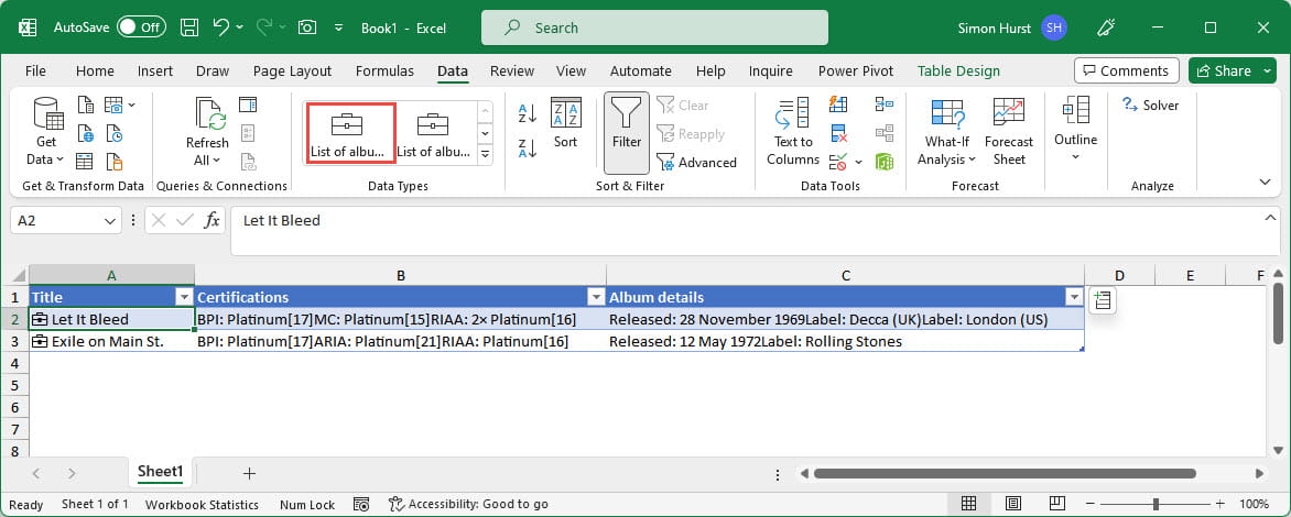
We can then publish our report to an appropriate Workspace and, the next time we restart Excel, the featured table should show up as one of the options in the gallery of Data Types:

The ‘Tell me more’ link opens the Help pane with further details and an introductory video.

We’ll start by creating a Table in an Excel worksheet. To start with, we will have a single column with the heading Post and enter a couple of possible Excel article content subjects. The detailed help explains how search terms are matched, but it seems that, in our case, using more than one word is likely to prevent Excel finding a match with the contents of the Post column of our featured table. So, entering ‘Conditional Formatting’ into a cell resulted in no matches when the Data Type was applied, even though there are posts that do begin with ‘Conditional formatting’. Accordingly, we just entered the words Conditional and Number into our two cells.

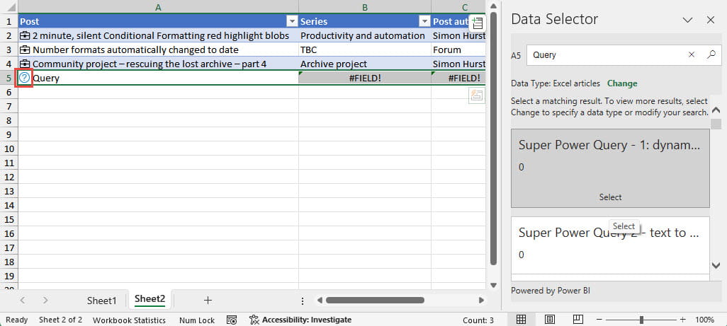
We can then select those two cells and click on the Excel articles organisational Data Type. Neither term is matched directly, but the Data Selector is displayed, allowing us to look through the matches for each term in turn. If you find the item you want, you can just click on the Select button to choose it:

Once we have selected our item for the first entry, the Data Selector pane will display the choices for the next entry.

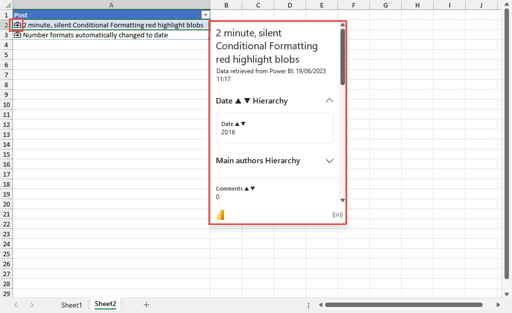
Here, we have selected posts for both of our search terms and then clicked on the Data Type icon at the left of our first cell to display the Data Card for our post. We can scroll to see all the available fields from our featured table:

We can also easily add columns to our Table to display other content in our featured table. We just need to have any of our Table cells selected and the Add Column icon will appear at the top right of our Table. Clicking on the icon will display all the columns from our featured table for us to choose from.

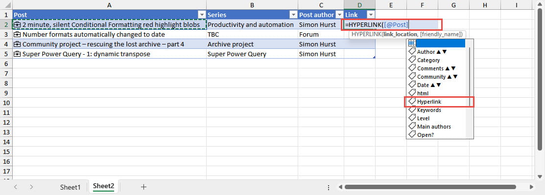
Once we have set the Data Type and added the columns that we want to include, because we have used an Excel Table, further entries will automatically be recognised as Data Types and the Data Selector can be used to select particular items. The other columns will then be completed automatically:

It is also possible to add columns that apply formulas to columns in the featured table, even if they have not been included as columns in the Excel Table. Our featured table includes the hyperlink to the actual Excel Community post on the Internet, but there would be a couple of drawbacks in just adding a column containing the hyperlink. Firstly, it would only appear as text and would not be directly clickable, and secondly it would be very long. Instead, we can add a custom column that uses the HYPERLINK() function to make the hyperlink text active and replaces the full hyperlink with the word ‘Link’. If we add a column and start a formula with the HYPERLINK() function we can click on cell A2 and we will be prompted to select a column from those in the featured table. We select the Hyperlink column:

We can then enter the second argument of our HYPERLINK() function as “Link”:

= Table.RenameColumns(#"Changed Type",{{"Service charge 1", "Charge 1"}})

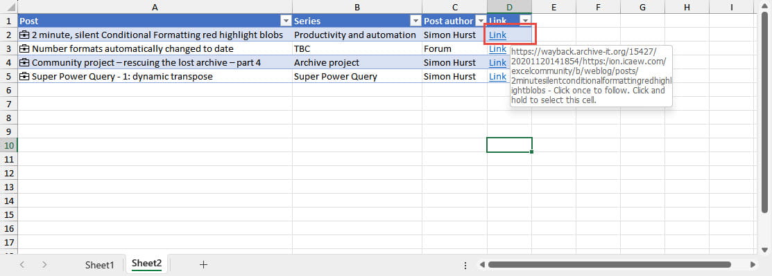
We now have a list of posts with additional information about the series they belong to and the author, and we can click on the Link hyperlink to open that article in a browser:

Our Data Type information is refreshable, so if the data in Power BI changes, we can right-click in our Data Type cell and choose refresh.

As we mentioned, the example we have used is perhaps untypical, but we could use this technique to provide access from within Excel to all sorts of organisational data such as supplier and customer details.

We could also use Power BI to extract information from online sources, such as a table on a web page, to create our own range of Data Types: