Avoid Column Name errors in Power Query

In Power Query, one of the biggest challenges is columns names changing in the source data.

We might be working with a downloaded month end report where the column headers are as follows:

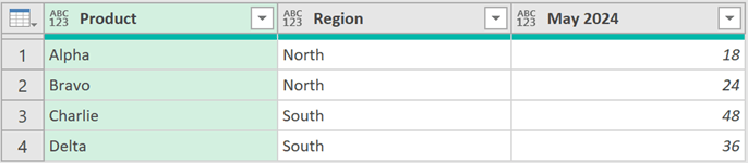
Everything looks fine until we realize there is a column header called May 2024. This will cause us some issues as some steps hard-code the column names into the M code.

Look at the example below, the Changed Type step has hard coded the May 2024 column name.

Next month, when the data changes and the column is called June 2024, the query will break.

Our goal, when using Power Query, is to ensure column names are not used in the M code, until we know those column names won't change.

In this post, we explore various ways to achieve this.

Useful M code functions

In this post, we use some useful M code functions which do not appear in the user interface. Let’s briefly explore those functions before we start.

Table.ColumnNames

Table.ColumnNames has the following syntax:

Table.ColumnNames(table as table) as list

It accepts a Table as an argument and returns the list of column names from that table.

Using the Promoted Headers step from the previous screenshot, we can use the following formula:

Table.ColumnNames(#"Promoted Headers")

which returns:

{"Item","Region","May 2024"}

The curly brackets ( {  } ) indicate this is a list. Therefore, we can access individual items in the list by referring their position.

In Power Query, lists are zero-based, therefore {0} is the first item 1, {1} is the second item, {2} is the third item, etc.

So, to refer to the May 2024 column by position, we could use:

Table.ColumnNames(#"Promoted Headers"){2}

Table.Combine

Table.Combine has the following syntax:

Table.Combine(tables as list, optional columns as any) as table

It accepts a list of tables and combines them into a single table. It stacks tables on top of each other, based on the common column names.

In this post, we are not looking at the optional columns argument of Table.Combine.

List.Zip

List.Zip has the following syntax:

List.Zip(lists as list) as list

It accepts a list of lists and outputs a different list of lists where each item has been matched by position.

For example:

= List.Zip({{"a","b","c"},{"x","y","z"}})

Returns:

{{"a","x"},{"b","y"},{"c","z"}}

OK, now we have a brief understanding of these M code functions, we are ready to start working through some scenarios.

Change column name by position

In the data, if the column name is always in the same position, we can change the name by using the Table.ColumnNames function.

Let’s start by renaming May 2024 to Value.

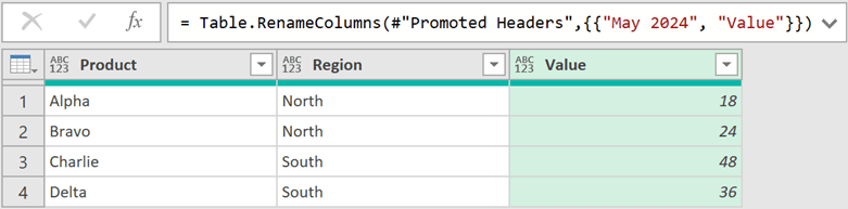
The formula bar shows:

= Table.RenameColumns(#"Promoted Headers",{{"May 2024", "Value"}})

Next, we change the M code to this:

= Table.RenameColumns(#"Promoted Headers",{{Table.ColumnNames(#"Promoted
Headers"){2}, "Value"}})

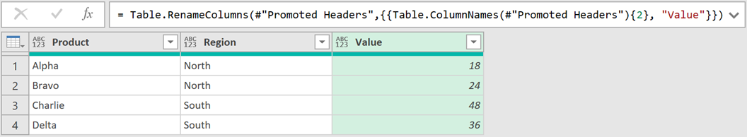
We no longer have a hard coded column name. When the source data changes to June 2024 there are no issues.

Expand columns dynamically

If we have a nested Table in Power Query, we usually want to expand it to see all the data.

However, by clicking the expand icon, Power Query uses the Table.ExpandTableColumn function, which hard-codes the column names.

The formula will be similar to this:

= Table.ExpandTableColumn(Source, "Data", {"Product", "Region", "April 2024",
"May 2024", "June 2024"}, {"Product", "Region", "April 2024", "May
2024", "June 2024"})

If any new column names are added to the source, they are not included in the expanded data.

To address this issue, we use the Table.Combine function.

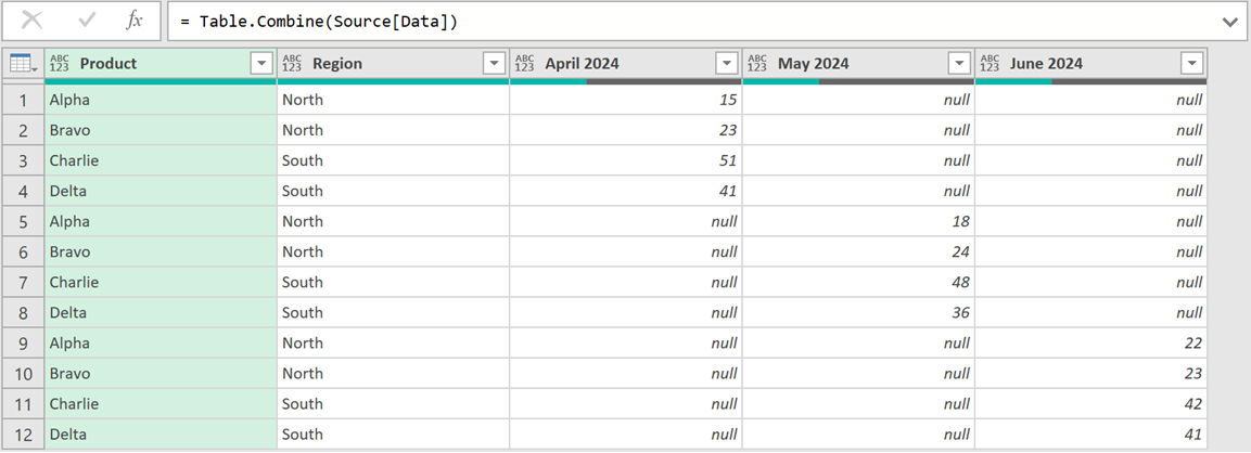
Instead of expanding the column, click the fx icon next to the formula bar and enter the following:

= Table.Combine(Source[Data])

• Source is the name of the previous step.
• Data is the column containing the nested tables.

The data combines into one Table, and no column names have been used.

Depending on your requirements, there are 2 possible issues here:

1. What if we want the previous column names which have now disappeared (e.g., Name, Item, Kind, Hidden)?
2. What if we don’t want each time period in a separate column?

Let’s tackle at each of these in turn.

Expand data and retain existing columns

Click the expand icon. Then change the auto generated formula as follows:

= Table.ExpandTableColumn(Source, "Data",
Table.ColumnNames(Table.Combine(Source[Data])))

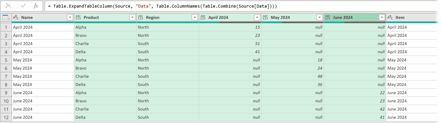
Now the data expands and retains the previous columns, and we have not referenced the column names.

Change column names in a nested Table

In the example above, we were able to expand the columns dynamically. However, April 2024, May 2024, are June 2024 were separate columns. We may want these stacking into a single column.

To do that, we can rename the columns inside the nested tables, before we expand them.

Before the step which expands the column, click the fx icon next to the formula bar and enter the following formula:

= Table.TransformColumns(Source, {{"Data", each
Table.RenameColumns(_,{{Table.ColumnNames(_){2}, "Value"}},
MissingField.Ignore), type table}})

• Source is the name of the previous step
• "Data" is the name of the column containing the nested table
• {2} is the column position to rename
• "Value" is the new column name we want to use

Adjust these elements to fit with your scenario.

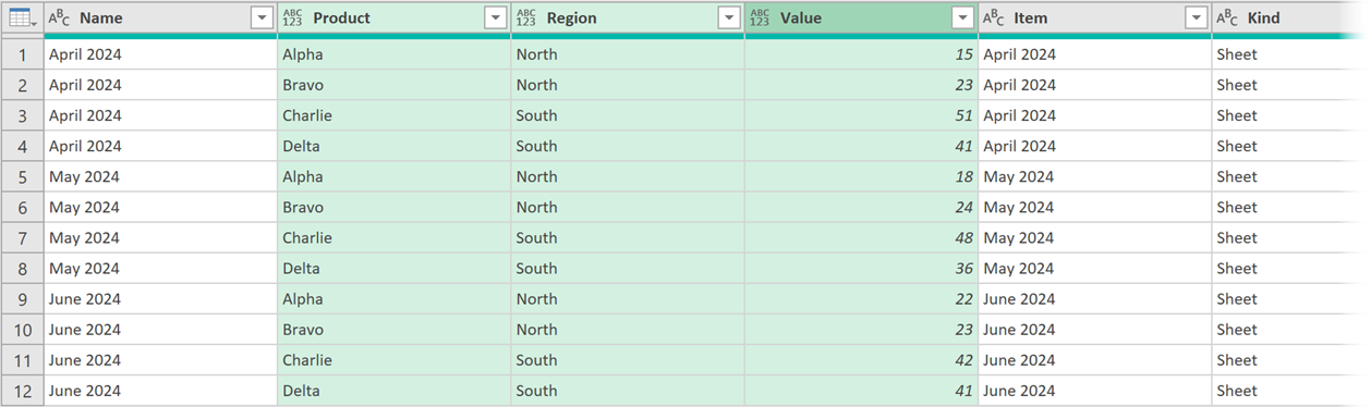
When we go back to the expand column step, everything expands into a single column.

Change column names based on a list

If column positions change, we can’t use the Table.ColumnNames method. We are forced to refer to them by name. For this we need create a list of old and new column names.

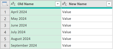
This query is called Rename List.

We could create the old name list dynamically, but that is outside the scope of this post.

In the main query, rename May 2024 to Value.

Notice how the generated M code is includes the column names in a list of lists.

{{"May 2024","Value"}} 

This is the same output at List.Zip.

Therefore, we can change the generated M code as follows:

= Table.RenameColumns(#"Promoted Headers",List.Zip({#"Rename List"[Old
Name], #"Rename List"[New Name]}), MissingField.Ignore)

• #"Rename List" is the table which contains the list of renames
• [Old Name] is the column which contains the columns to rename
• [New Name] is the column which contains the new names

Adjust these elements to fit with your scenario.

Now the columns are renamed based on the list.

If you need to rename the columns inside a nested list, use the following formula:

= Table.TransformColumns(Source, {{"Data", each
Table.RenameColumns(_,List.Zip({#"Rename List"[Old Name], #"Rename
List"[New Name]}), MissingField.Ignore), type table}})

• Source is the name of the previous step
• "Data" is the name of the column containing the nested table
• #"Rename List" is the table which contains the list or renames
• [Old Name] is the column which contains the columns to rename
• [New Name] is the column which contains the new names

Adjust these elements to fit with your scenario.

Dealing with pivoted data

So far, we have use data in first normal form. But if the data is pivoted, we must first unpivot before even thinking about the column names.

Here is the example data:

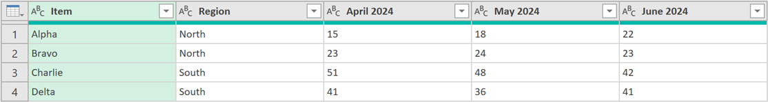
As always, we don’t want to hard code any column names that might change.

Select the column names to pivot on (Item and Region in our example). These are usually the column names which will not change.

From the ribbon, click Transform > Unpivot (drop down) > Unpivot Other Columns.

The data now looks like this:

The M code generated for this step is:

= Table.UnpivotOtherColumns(Source, {"Item", "Region"}, "Attribute",
"Value")

The only column names hard coded relate to column names that will not change. So, this will also avoid future column errors.

And yes, we can apply this to a nested table using the following formula:

= Table.TransformColumns(Source, {{"Data", each
Table.UnpivotOtherColumns(_, {"Item", "Region"}, "Attribute", "Value"),
type table}})

• Source is the name of the previous step
• "Data" is the name of the column containing the nested table
• {"Item", "Region"} is the list of column names to unpivot on

Adjust these elements to fit with your scenario.

Conclusion

In this post, we have seen why column names cause so many issues.

Then, we looked at various techniques for handling column names dynamically. No matter the structure of your source data, it’s just a matter of applying the right techniques to avoid the common column name errors.