Creating a dynamic lead schedule

We have covered the FILTER function a few times, most notably in Tip #437 - Revisiting dynamic arrays and Tip #443 - Next level FILTERing. I won’t go into much detail, but the function is defined using the following =FILTER(array to filter, one or more conditions, [default value]).

We’ll start with a categorised trial balance like the example below, this is in an Excel Table called TBInput.

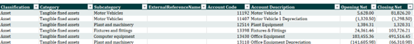
We want it in a table to make the formula more readable and to deal with differing amounts of data each time we use our lead schedule.

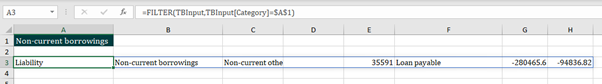
Using the formula =FILTER(TBInput,TBInput[Category]=$A$1) We can pull back the contents of the table where the category matches the text in A1. You can see from the blue outline around the cells this is a dynamic array formula which spills into adjacent cells. If you get a #SPILL! error make sure there is enough space for your formulae to work (see Tip #437 to learn more about this). We can add a default value of blank by completing the final parameter i.e. =FILTER(TBInput,TBInput[Category]=$A$1,””), this helps us deal with missing data covered later.

This works but what if we want multiple categories or a selection of subcategories. For this we can use VSTACK, =VSTACK(array1,[array2],…). Simply comma separate a list out the various filters you want to apply. It’s the equivalent of using OR logic within the filter.

=VSTACK(
TBInput[#Headers],
FILTER(TBInput,TBInput[Category]=”Cost of sales”,””),
FILTER(TBInput,TBInput[Category]=”Distribution costs”,””),
FILTER(TBInput,TBInput[Category]=”Administrative expenses”,””))

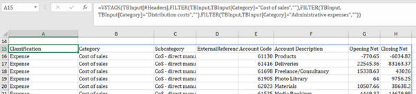
As shown, this pulls in the column headers from the TBInput table followed by any TB codes in Cost of sales, Distribution or Administrative expenses.

This typically isn’t in the format you’ll need but this is where CHOOSECOLS can help.

CHOOSECOLS as the name suggests allows you to choose which columns (and order) your data is returned in.

The formula is used as shown =CHOOSECOLS(array,col_num1,[col_num2],…)

In this case the array will be our filtered TB formula from above and then you can list which columns you require with comma separated numbers. You could theoretically use a match formula to provide column numbers but given the use case is a lead schedule my assumption is that the source data will be consistent in format.

If we wrap our previous formula in =CHOOSECOLS(PreviousFormula,5,6,7,8,2,3) this defines the look of our returned data as shown:

We now need to adjust our formula to better deal with missing data. On our example above we don’t have any Distribution costs. If we missed the default value parameter in our filter section, we’d get a #CALC! error. Assuming you’ve done that instead you’ll get a line of #N/A.

To remove this, to allow SUM formula or similar to function properly we’ll need to enclose the whole formula with =IFERROR(PreviousFormula, ””) to replace the N/A with a blank cell.

The whole formula is now:
=IFERROR(
CHOOSECOLS(
VSTACK(
TBInput[#Headers],
FILTER(TBInput,TBInput[Category]="Cost of sales",""),
FILTER(TBInput,TBInput[Category]="Distribution costs",""),
FILTER(TBInput,TBInput[Category]="Administrative expenses","")),
5,6,7,8,2,3),
"")

Creating dynamic dropdown options

These have been covered before in Tip #219 - Nested dropdowns using multiple named ranges and utilising the INDIRECT formula to switch between the options.

Using the newer dynamic array formula introduced above we can create similar nested dropdowns without data preparation. In this example we’ll start with the same TBInput table.

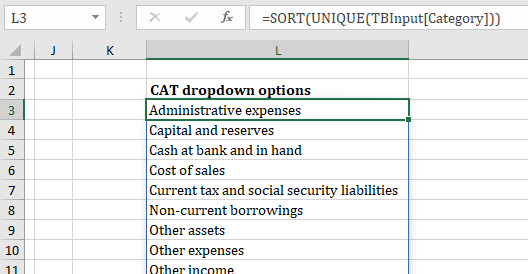
We can create a list of sorted unique categories from our TB using =SORT(UNIQUE(TBInput[Category])). Both SORT and UNIQUE are covered in Tip #437 - Revisiting dynamic arrays.

We can then point a named range at the originating cell. If we edit the named range, we can add a hash symbol to the end of the reference and the named range will dynamically update too.

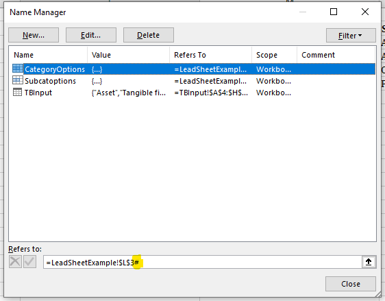
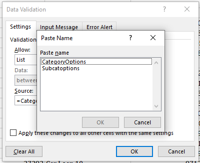
When you are setting the data validation select List then after clicking into the Source box press F3 to be able to select named ranges as your defined cell options:

Now we can create the nested dropdown using the same combinations of formulae as seen above.
=VSTACK(
"All",
SORT(
UNIQUE(
CHOOSECOLS(
FILTER(TBInput,TBInput[Category]=$A$2,""),
3))))

FILTER – We can filter the TB to all rows where the category has been selected by our original dropdown in A2.

CHOOSECOLS – We can pull back only the subcategory column (column 3 in this case).

UNIQUE – Remove duplicates to a list of unique options.

SORT – Sort alphabetically.

VSTACK – This allows us to inject an “All” option at the top of the list.

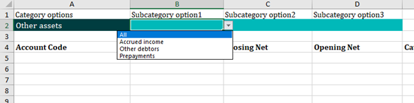
This also needs setting up as a named range creating with a # on the end of the reference. Setting up another dropdown menu allows a dynamic list of options based on the previously selected dropdown but with our additional All option added:

Going back to the dynamic lead schedule example we can update our hard typed categories into subcategories looking at the results of our dropdowns. I’ve then added an IF formula to override the subcategory filters to look at the whole category if All is selected in any dropdown.

=IFERROR(
CHOOSECOLS(
IF(COUNTIF(B2:D2,"All")>0,FILTER(TBInput,TBInput[Category]=$A$2,""),
VSTACK(
FILTER(TBInput,TBInput[Subcategory]=$B$2,""),
FILTER(TBInput,TBInput[Subcategory]=$C$2,""),
FILTER(TBInput,TBInput[Subcategory]=$D$2,""))),
5,6,8,7,2,3),
"")

• Download an example of the dynamic lead schedule