One of Excel’s most significant updates this decade is without a doubt the new GROUPBY and PIVOTBY functions, these can replicate PivotTables functionality through formulas, so here I will compare and contrast both methods whilst providing possibly the most complete guide on the internet currently of GROUPBY.
Key differences
- GROUPBY & PIVOTBY functions refresh automatically, PivotTables do not
- GROUPBY & PIVOTBY can return additional functions like a concatenated list of values
- GROUPBY & PIVOTBY can create any chart type, PivotTables have limitations
- PivotTables are easier to create without understanding coding/formulas
- PivotTables group dates and continuous variables for easy aggregation by month/age range etc.
This video showcases some key aspects where the functions outshine PivotTables:
Aggregations via PivotTables & GROUPBY
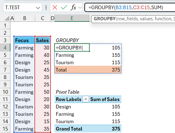
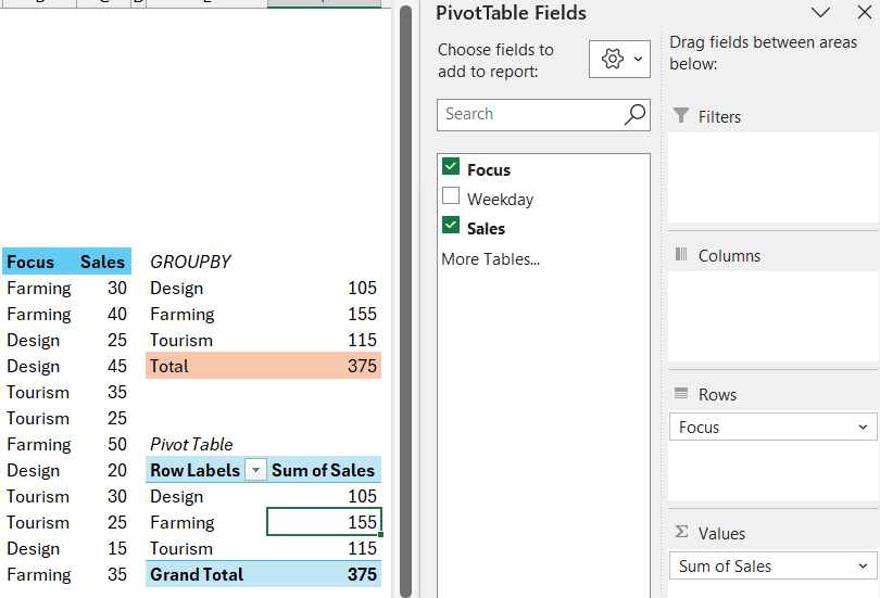
PivotTables can aggregate by category without formulas or manual filters. In September 2024, Excel released two new functions to the Microsoft 365 Current Channel which can also aggregate by category GROUPBY and PIVOTBY.In this example the sales are summed by category leading to the same results using both methods. SUMIFS has been a long-standing formula which could return the individual results for each category, but with GROUPBY, you can write a single formula to generate the same output analysis table. You can download the accompanying workbook here to follow through the examples.


Using GROUPBY
GROUPBY replicates a one-dimensional PivotTable (eg, Sales by region), you specify the row field, the values field and the aggregation type as minimum. The full syntax is below [inputs in square brackets are optional as usual]:
GROUPBY(row_fields, values,function, [field_ headers], [total_ depth], [sort_ order], [filter_ array], [field_ relationship])
In this example, I specify the focus column being the row fields, Sales is the Values fields and SUM is the function to aggregate by, anyone comfortable writing a SUMIFS function shouldn’t struggle with using GROUPBY.
This video discusses the different inputs:
Using PIVOTBY
PIVOTBY(row_fields,col_fields,values,function,[field_headers],[row_total_depth],[row_sort_order],[col_total_depth],[col_sort_order],[filter_array],[relative_to])
This function is similar adds column fields, note that even though they have no square brackets row-fields and col_fields can be left blank. You also get total and sort options for both rows and columns. The last input is discussed when I mention the PERCENT OF aggregation. A key difference though is I don’t particularly like how the field headers are displayed in PIVOTBY so I usually don’t display these.
Built in aggregation functions
Aggregations in both the formula version and PivotTables are here:
- SUM, COUNTA and AVERAGE are the most commonly used in both
- The less frequently used options in both include min, max, product, count numbers, variance, standard deviation (each for sample or population)
- PERCENTOF in GROUPBY is equivalent to show % of totals, other “Show values as” options
- In PIVOTBY (but not in GROUPBY), you can switch between % of total, % of row total, % of column total or % of parent total (either in row or column). Note that you may leave row fields or column fields blank in PIVOTBY if you want a one-dimensional PivotTable that does % of parent totals. More on the specifics of that are on this video:
Built in aggregations only in GROUPBY
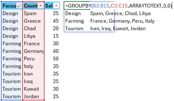
- ARRAYTOTEXT is one of my favourite aggregation types, it creates a comma separated list. This type of analysis has been so essential to me in the past that I would frequently use workarounds to get these with extremely long formulas, so I love that its built into GROUPBY. CONCAT is another option in GROUPBY which joins the text without a separator, so it is less practical
- MEDIAN and MODE.SNGL are two extra statistical measures which are in GROUPBY but not PivotTables, I’ve felt the need for these in the past but not regularly.
Built in aggregations only in PivotTables
- PivotTables provides multiple options under “Show Values As” which GROUPBY/PIVOTBY do not, including ranking, difference from previous, running totals and more. Personally I very rarely use these.
Aggregations which ignore duplicates & other custom ones
The methodology for these differ:As well as the built-in functions, the 17th function on the list for GROUPBY & PIVOTBY allow you to code your own aggregation to make anything that you want. To use LAMBDA in this case you can write =LAMBDA(x, function combination (x)). The two ways that I use it the most are for unique aggregations, as shown in this screenshot and explained below:

- =GROUPBY(Field Column, Values column, LAMBDA(x,COUNTA(UNIQUE(x)) will return a distinct count
- =GROUPBY(Field Column, Values column, LAMBDA(x,ARRAYTOTEXT(UNIQUE(x)) will return a distinct comma separated list of the values
- You can use LAMBDA in the same way to create other aggregations or more complex measures like running totals etc. Using PivotTables, you must tick the box “Add this data to the Data Model” to make be able to choose a Distinct Count from the aggregation list in a PivotTable.
Using PivotTables, you must tick the box “Add this data to the Data Model” to make be able to choose a Distinct Count from the aggregation list in a PivotTable.

Headers, totals, formats and layouts
After the 3 optional inputs in GROUPBY the rest are all optional. Inputs 4 and 5 are shown below.
4. [field_ headers]: Choose between options for headers not selected, headers selected but don’t show in output or show in output.
5. [total_ depth]: Choose to show grand totals or sub totals, subtotals are only relevant when using multiple fields (see below). The PIVOTBY function has separate inputs for row totals and column totals
With PivotTables, you can click a cell inside the Pivot, then click Pivot Tables Design choose which options you’d like for subtotals, grand totals different styles and layouts. You get more flexibility by clicking Analyze tab then options. You can also set your preferred default PivotTable by clicking File > Options > Data > Edit Default Layout on the top.

There is no doubt that Pivots offer more granular formatting options, but I personally sometimes still feel PivotTable formatting not flexible enough than using cell by cell formatting, plus the labels used for the “Report layout” are not very intuitive to me.
Sorting
GROUPBY has a sort order as the optional 6th input. To sort by the 2nd column in ascending order type 2, or to sort by the 3rd column in descending order type -3. PIVOTBY has row sort order and column sort order options. To do a multi-level sort, type the instructions in {curly brackets}.
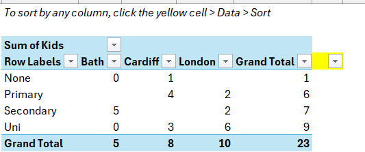
PivotTables can be sorted by clicking on the filter dropdown then click to sort or choose more options. You can also sort manually using drag & drop, or a secret trick to sort by any column when you have column fields active is to select the cell just to the top right of the PiovtTable and then the filter/sort icons will show up on every column, as shown here:
Filtering
GROUPBY and PIVOTBY have an optional input for filtering, entering [Country]=”UK” could filter only the UK entries or entering [Product]< />”Total” could filter out total rows.
PivotTables allow you to filter in 3 ways:
- To filter by a field in the PivotTable, click the filter dropdown
- To filter by a field not in the PivotTable, use the Filter quadrant
- Add a slicer for a more user-friendly filter. Note that slicers can be used with GROUPBY via a workaround discussed here.
Using multiple fields
This is where PivotTables are far easier, you put a tick mark next to whichever column you want in rows, columns or values and drag the same column into Values if you would like to do different aggregations (eg, SUM of sales, % of total of sales by category and Average of Sales).
When using multiple fields with GROUPBY or PIVOTBY:
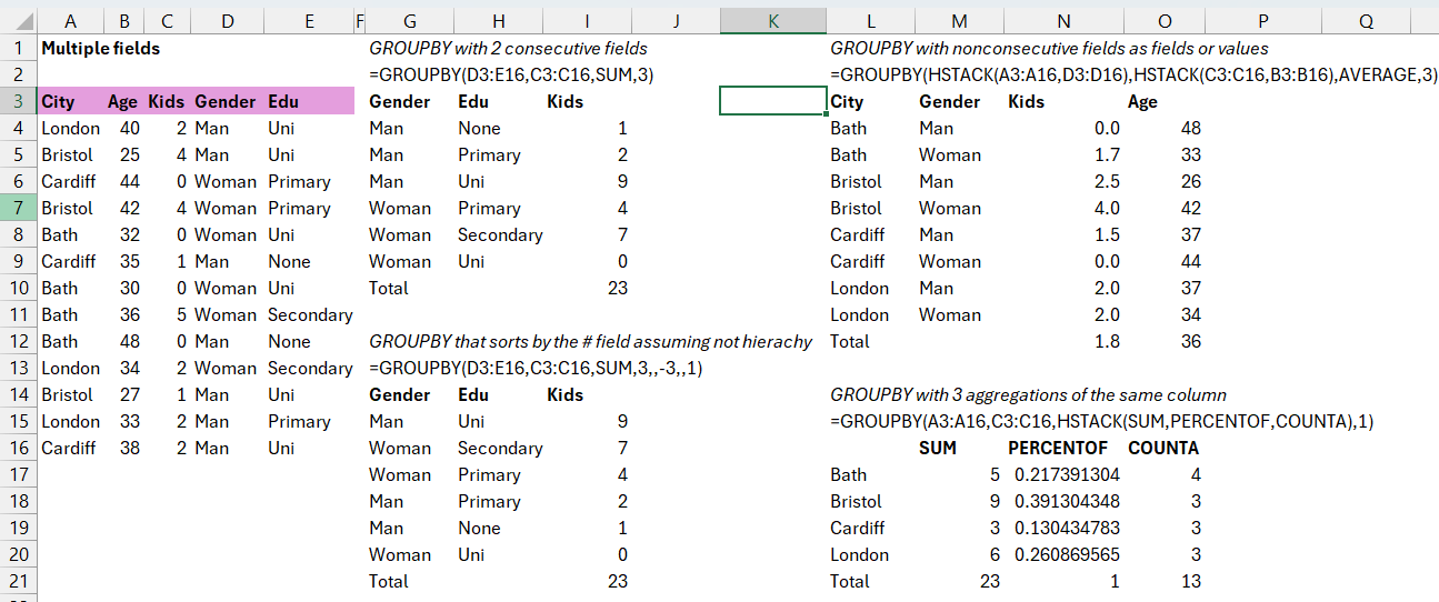
- If the columns are consecutive, you can select multiple columns in your formula input, eg, =GROUPBY(D3:E16,C3:C16,SUM,3)
- If the columns you want in row fields are non-consecutive or you’d like to reorder the columns, you need to add an additional function, usually I use HSTACK which stacks arrays horizontally. =GROUPBY(HSTACK(A3:A16,D3:D16), C3:C16,AVERAGE,3)
- If the columns you want in values fields are non-consecutive or in a different order, you can again use HSTACK, this formula has two row fields and 2 value columns. =GROUPBY(HSTACK(A3:A16,D3:D16),HSTACK(C3:C16,B3:B16),AVERAGE,3)
- If you’d like to perform different aggregations on the same values column, you can use HSTACK on the third input for function, an example is =GROUPBY(A3:A16,C3:C16,HSTACK(SUM,PERCENTOF,COUNTA),1)
- The default means sorting by the values column will keep each group together but If you’d like to sort as a regular table (for non hierarchal data), the final input in GROUPBY allows that. =GROUPBY(D3:E16,C3:C16,SUM,3,,-3,,1)
Charts & slicers
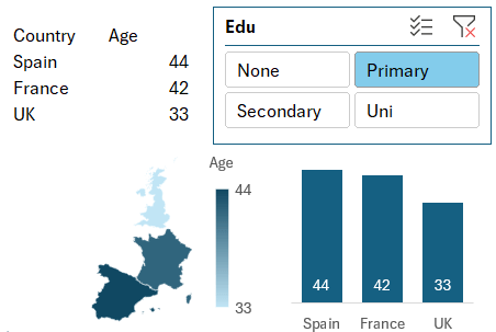
GROUPBY and PIVOTBY create a dynamic array, which changes in size depending on the data and charts can be based on dynamic arrays, and the functions can actually produce several charts which PivotTables cannot. Here are some key tips:
- Charts from GROUPBY should show headers and no totals
- Charts from PIVOTBY should show no headers and no totals
- You can create any chart from the functions, whereas PivotTables cannot be the source for newer charts eg, map charts, box & whisker, waterfall, funnel, tree map or sunburst charts
- To link GROUPBY to a single select slicer, create a PivotTable with the same single field in rows and in slicer, then link the PivotTable output cell to GROUPBY’s filter input. To create more advanced slicer connections, read this other ICAEW article by Mark Proctor - Using slicers with PIVOTBY, GROUPBY and FILTER
- Timelines don’t work on GROUPBY
More information and a demo is shown in this video:
Other aspects
| Aspect | GROUPBY/PIVOTBY | PivotTables |
|---|---|---|
| Refresh | Automatic | Manual |
| Show values in rows (multiple aggregations) | Not possible | Drag Values into rows |
| Grouping continuous fields (dates or numbers) | Must be done in source table | Right click date field > Group |
| Pivot analysis from multi table data model | Not possible | Use Power Pivot |
| Custom formulas | Use LAMBDA | Calculated fields or add to the data model and use DAX for more options |
| Compatibility | Excel 365 on Online only | PivotTables work on all versions but PowerPivot isn’t available on Mac or some versions of Excel 2016 or older. |
Versions
Subscribers on the Current Channel have access, those on Monthly Enterprise Channel should in theory get it in the next couple of months yet subscribers to the Semi-Annual Channel likely will not have access until July 2025. To check which channel you are on, click File > Account to check which version you are on. Excel Online has the functions available.
Anyone with a perpetual version of Excel Desktop (Office 2024, 2021, 2019, 2016 etc.) or Google Sheets will not have access to GROUPBY or PIVOTBY.
Archive and Knowledge Base
This archive of Excel Community content from the ION platform will allow you to read the content of the articles but the functionality on the pages is limited. The ION search box, tags and navigation buttons on the archived pages will not work. Pages will load more slowly than a live website. You may be able to follow links to other articles but if this does not work, please return to the archive search. You can also search our Knowledge Base for access to all articles, new and archived, organised by topic.

