Introduction

Last time, we looked at calculating the total number of presents donated over the 12 days of Christmas according to the festive song. As part of creating the required formula, we used the MAKEARRAY() function to create a visual representation of the calculation in a 12 by 12 matrix:

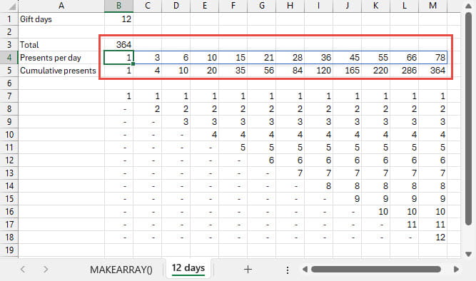
As useful as the matrix might be in visualising the problem, it could certainly be improved by replacing the dull numbers with appropriate pictures. It would be possible to do this using pictures in cells, and formulas, but it would be a bit cumbersome. Instead, we could make a relatively simple addition to our MAKEARRAY() formula. We are going to use the INDEX() function which can return elements of a set, such as cells in a column, by position.

First of all, we need to create our twelve pictures. We have used Microsoft Paint with its new generative AI capabilities to create the pictures, with impressive results for the most part, and save them.

We have then used the Insert Ribbon tab, Illustrations, Pictures, Place in Cell option to choose This Device…

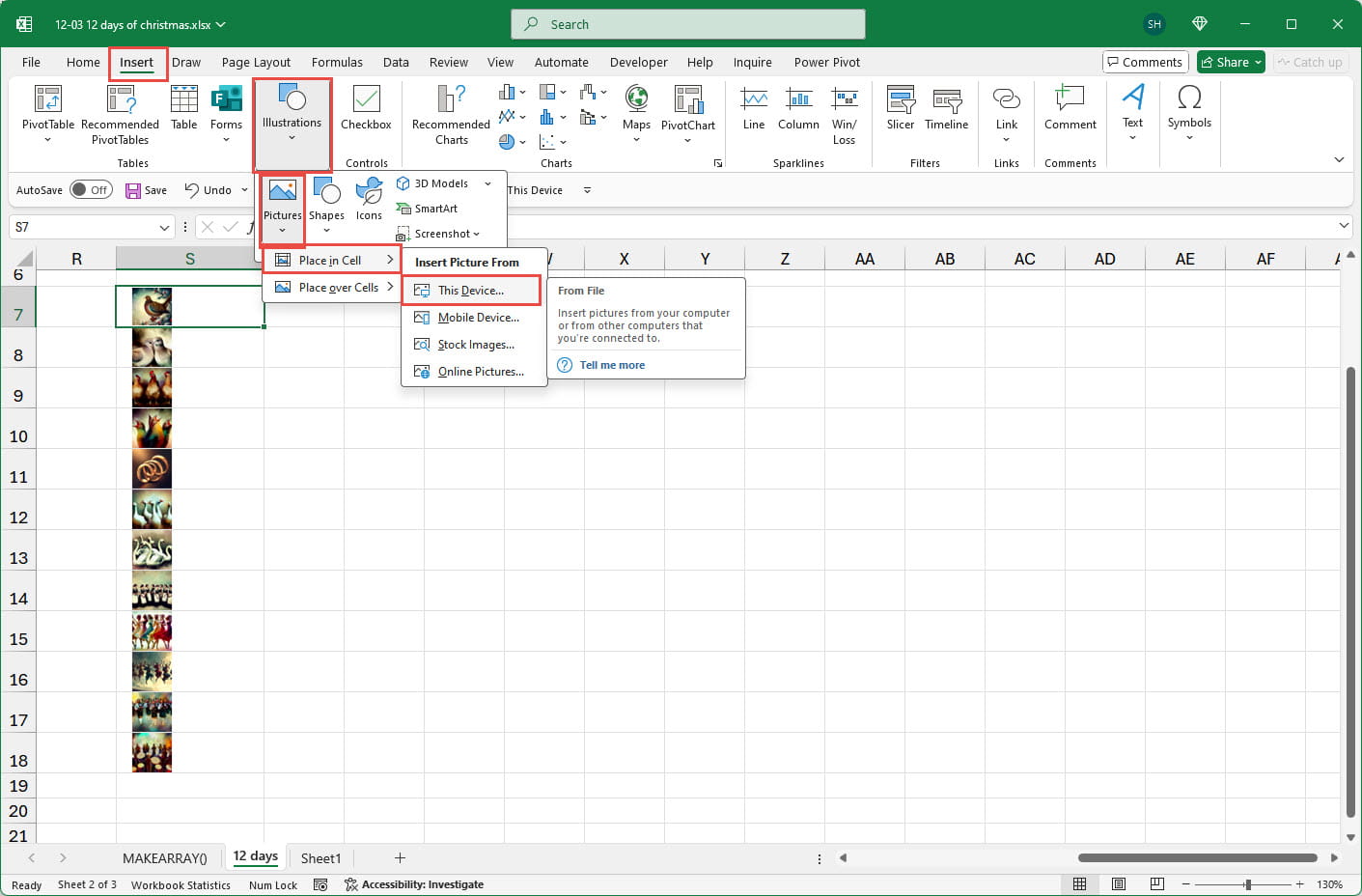
INDEX() allows us to refer to the cells containing the pictures by their position in the column, using the numbers 1 to 12 – the same numbers that we already have displayed in our grid.

The first argument of the INDEX() function is the range of cells containing the pictures. The second INDEX() argument is the index number representing the position, in our case this is a number from 1 to 12 to correspond with the number of cells in our range. We are using our MAKEARRAY() function to provide these numbers in our grid format:

=INDEX($P$7:$P$18,MAKEARRAY(GiftDays,GiftDays,LAMBDA(r,c,r*(c>=r))))

Unfortunately, this doesn’t quite work. Although the numbers from 1 to 12 do work, and do put the pictures in the correct places, where our MAKEARRAY() function returns 0, INDEX() still seems to return picture 1:

In fact, INDEX(), with the position number set to 0, actually returns the entire array of cells and, because this is already part of an array, it can only display the first item in the array. We can see this by using the INDEX() function on its own:

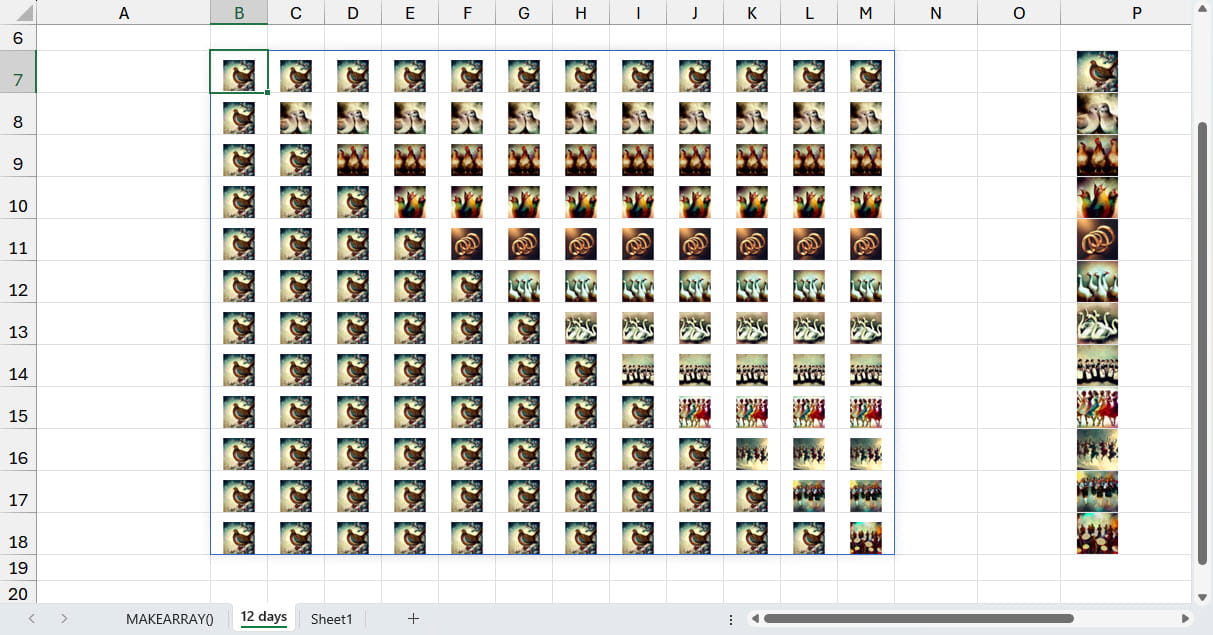
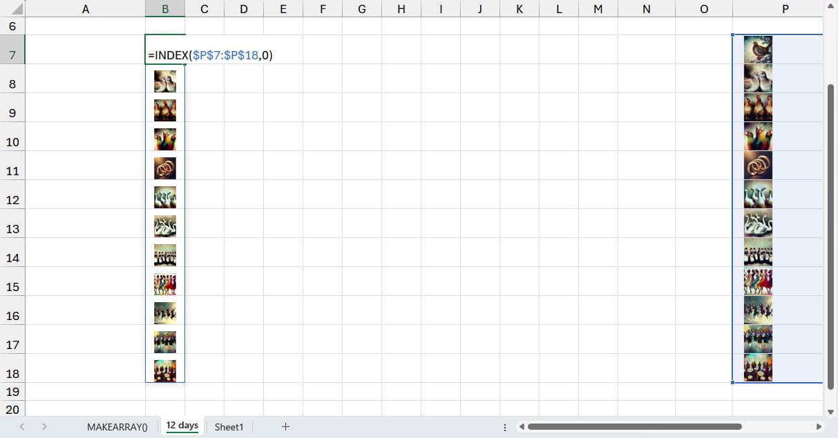
One solution is to add 1 to each index number so that our grid contains the numbers 1 to 13, rather than 0 to 12. We can then extend our picture array to include a blank cell at the top of the array. The cells that previously displayed 0 will now display 1. Used as part of INDEX(), 1 will now return the contents of the empty cell, with index numbers 2-13 returning the pictures for days 1 to 12.

=INDEX($P$6:$P$18,MAKEARRAY(GiftDays,GiftDays,LAMBDA(r,c,r*(c>=r)+1)))

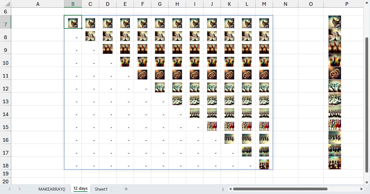
We now have our grid of gift pictures and potentially the answer to several other Christmas quiz questions.

Not just for Christmas…

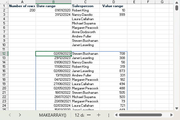
This technique has a wider application than answering Christmas quiz questions. Using INDEX() with a list within a dynamic array formula can play a part in generating random data for testing or similar purposes. In this example, we have used a variety of Excel dynamic array formulas to populate a range of cells with random values:

=HSTACK(RANDARRAY(A2,1,B2,B3,TRUE),INDEX($C$2:$C$10,RANDARRAY
(A2,1,1,COUNTA($C$2:$C$10),TRUE)),RANDARRAY(A2,1,D2,D3,TRUE))

Additional resources

You can explore all aspects of Excel, including other Christmas special series, in the ICAEW archive:

• Excel archive