Excel Tables – so much more than just a pretty format

When Tables were first introduced into the Windows versions of Excel in Excel 2007, many people saw them as another Excel formatting ‘gimmick’. This view was supported by the inclusion of the Format as Table command in the Styles group of the Excel Home Ribbon tab. However, it soon became apparent that Tables were much more important than that, and that they had a significant role to play in many aspects of automating Excel.

This is the story so far:

• Creating Excel Tables
• The Tables superpower – auto expansion
• Setting Table size manually and the role of Tables in automating Excel
• More automation techniques, including the use of Data Validation and Dynamic Arrays
• The Table Design Ribbon tab options
• From Table to Dashboard
• Structured References part 1
• Structured References part 2
• Sorting, filtering, Sparklines and check boxes

Introduction

The ultimate product of a Power Query query, or related set of queries, is often a linked Table on an Excel worksheet. In this, concluding, part of our Tables series we will look at some of the issues and opportunities that are particularly relevant to the Tables generated by Power Query before looking at an example that brings together many of the techniques we have covered in the series and also a significant Table drawback.

Linked Tables and extra columns

When a Table linked to a query is refreshed, the number of columns, as well as the number of rows, might change. It can be important to understand how a change in the number or columns can affect columns that you have added to that Table in the worksheet itself.

Before we start looking at entire columns, it’s vital to understand that any changes made to the contents of the part of any table that is linked directly to a query will be overwritten when the query is refreshed. This might seem obvious but, when a query, and the data upon which that query is based, are both in the same workbook, it can be all too easy to accidentally make a change to the result of the query, rather than to the underlying data, with the change being overwritten the next time the query refreshes.

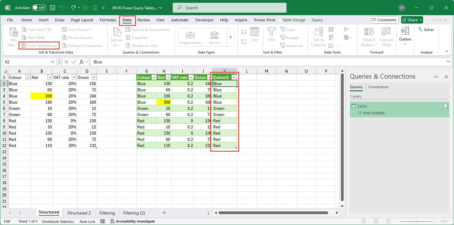
In this example, we have used the Data Ribbon tab, From Table/Range command to load our Table data into a query. We have then used the Power Query ‘Close & Load to…’ command to load our query output next to the original data. We have placed the query Table adjacent to the original data just to make it easier to see what is going on. Generally, it would be much better to place the output Table in its own worksheet. Having created our query and output Table, we have added a column to the output Table and typed in the same text as is in the original Colour column. We have also made an edit to the underlying data, and to the output Table contents, after the Power Query output Table has been created:

We will now edit our query to sort the output Table by the value in the Net column, before loading the revised query back into the worksheet:

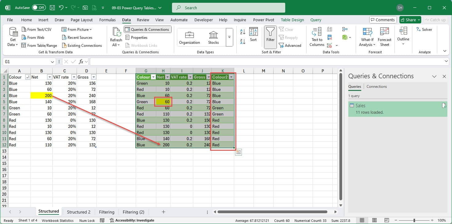
As you can see, our added column cells have not changed position and our entries no longer line up with the contents of the original Colour column. For this reason, trying to combine Power Query output columns with data entry columns in the same Table can be fraught with danger. Even if you use an index column to help preserve the sort order, there is always the chance that a change in the underlying data, or the application of a filter for example, could destroy the integrity of the data, with the data entries no longer being on the same rows for which they were originally entered.

With regard to the edited cells, as anticipated, the change made to the underlying data in cell B4 is reflected in our output Table where it is in cell H12. However, the change made in the output Table itself, in cell H5, has been overwritten by the original data when the query has been refreshed during the load process.

Although there is very little that you can’t do to manipulate data within Power Query, there are some circumstances where it can be more straightforward to add a calculated column to an output Table.
Here, we have added a formula column to the right of our existing Table and it is automatically incorporated into our Table. We have inserted another formula column in the Middle of our Table by right-clicking on the column heading to the right and choosing Insert. It might not be immediately obvious how to add a column to the Left of our Table as, unlike a column at the right of a Table, just typing in a column heading in the column to the left of our existing Table will not automatically expand the Table dimensions to include it. Instead, we can right-click in the current leftmost Table column and choose Insert, Table Columns to the Left.

To check what happens with rows, we have added one row within the Table and then another row that is outside of our Table:

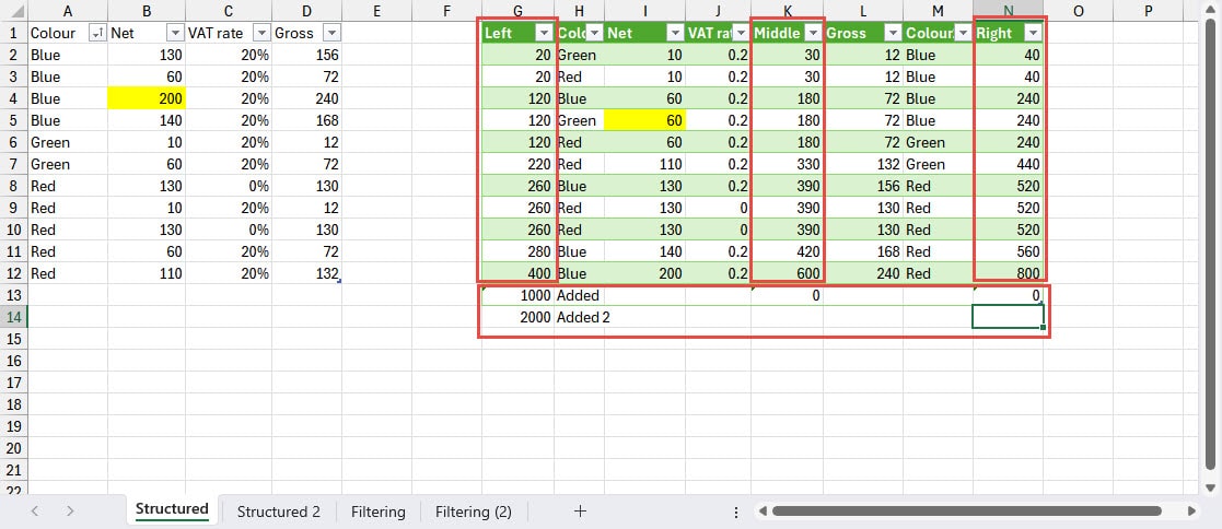
As well as adding our new Table columns and entering a formula in each one, and adding our two new rows, we have added a new column within our Power Query and moved it between our Net and VAT rate columns. We have also added two rows at the bottom of our original data Table.

When we Refresh the query behind the Table, we can see that our added columns are preserved and the formulas are copied down to the added rows. For the rows added at the bottom of our output Table, we can see that the row added as part of our Table has been removed and overwritten by our new rows whereas the cell entries made underneath, but outside of the Table, have been moved down as the output Table has expanded. We can also see that rows added in the column of text entries are empty:

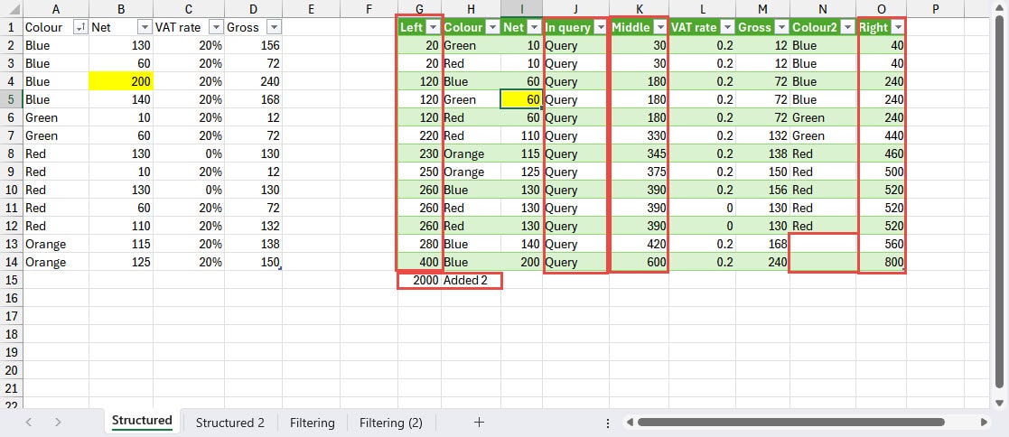
It is usually preferable to keep linked Tables that are subject to expansion or contraction on their own worksheets in order to avoid problems with Tables clashing with each other as they expand or contract. However, there are circumstances where it is useful to be able to see refreshable Tables on the same worksheet. In an earlier article, we explored this issue in more detail:

• Multiple Excel Tables in a single worksheet – avoiding Cell Clash

Tables, power query and formatted accounts

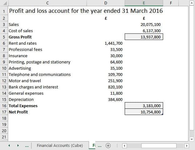
Another series of articles looking at Power Query and Tables combined ended up using several Table features to format an Excel Table based on Power Query to create a formatted set of accounts:

• Experimental Excel - from Power Query table to formatted accounts
• Experimental Excel - Mission Accomplished or Mission Impossible?

It’s not all good

While looking at some previous articles, its worth mentioning a long-running issue with Excel Tables: the way that Tables work with worksheet protection. Principle 20 of the ICAEW 20 Principles for Good Spreadsheet Practice recommends that, once reviewed and checked, all formulas in spreadsheet should be locked, and each worksheet protected, to reduce the chance of formulas being changed inadvertently. Unfortunately, as soon as you turn on worksheet protection, it becomes impossible to add rows to any Table on that worksheet, without the use of advanced features such as using programming code. Given the benefits of using Tables for simple data entry, combined with calculated columns to process new data as it is added, this is a significant drawback:

• Excel Tables bug hits key milestone

Next time…

This time, there is no next time in the Table series (for a while at least). I hope that you have found the series useful and, if you hadn’t previously discovered the extensive capabilities of Excel Tables, that you have been inspired to make more use of them.

Conclusion

• You can explore all aspects of Tables, and a great deal more, in the ICAEW archive