Simple but effective, part 3 – extending Tables

Excel Tables – so much more than just a pretty format

When Tables were first introduced into the Windows versions of Excel in Excel 2007, many people saw them as another Excel formatting ‘gimmick’. This view was supported by the inclusion of the Format as Table command in the Styles group of the Excel Home Ribbon tab. However, it soon became apparent that Tables were much more important than that, and that they had a significant role to play in many aspects of automating Excel.

Having looked at different methods of turning ranges of cells into Tables in part 1, and seen how Tables automatically expand to incorporate new rows and columns in part 2, this time we will consider some ways to change the dimensions of a Table manually.

Resizing a Table

A resize handle appears at the bottom right-hand corner of an Excel Table. This can be dragged down or right to extend the range of cells that the Table includes and can also be dragged up or left to exclude existing rows and columns from the Table. Alternatively, the Properties group of the contextual Table Design Ribbon tab includes a Resize Table command. Clicking this command displays a dialog that allows a range of cells to be typed in or dragged. The range needs to use the same header row as the existing Table:

Inserting Rows and Columns

If you right-click a cell in the data area of an existing Table and choose Insert, you will have the option of inserting a Table Column to the Left (and, if you click in a cell in the rightmost column of the Table, to the Right); or a Table Row Above (and, if you click in a cell in the bottom row of the data area of the Table, Below):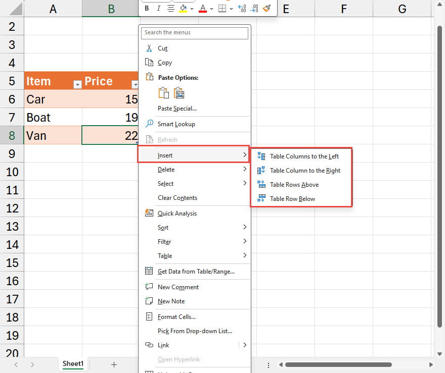

This technique can be particularly useful if you need to add a column to the left of an existing Table that is created as the output of a Power Query.

Extending Tables using the Tab key

Pressing the keyboard Tab key when a Table cell is selected will select the next cell in the Table horizontally and, when you get to the rightmost column, vertically. Once you get to the bottom right-hand corner cell, continuing to press the Tab key will insert new rows. Note that when the Total Row is included using the option in the Table Style Options group of the Table Design Ribbon tab, the new row will be inserted above the Total row and the Total row will be moved down to accommodate the new row or rows.

Using Tables to automate data processing

Having looked at the various ways of changing Table dimensions, we will consider how this can help automate the journey from a raw table of data to a formatted report. Generally, creating a formatted report based on a table of data will require data to be summarised. For example, the sales values in a table of individual sales invoices could be summarised by product, allowing a report to include up-to-date product sales totals. Because a formula reference to an entire Table column will automatically include all of the rows in that column whether the Table expands or contracts, an Excel formula would be able to adjust automatically as data is updated to include new invoices: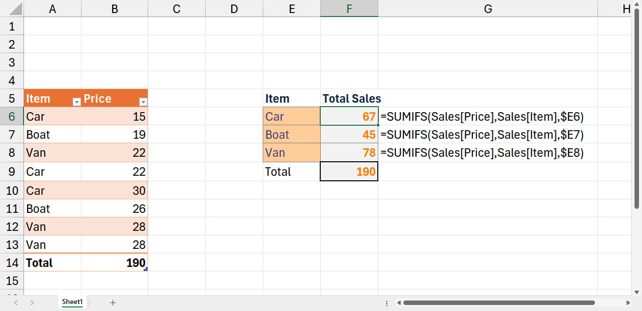

In this example, we are just using the existing data in the Table, but if we needed to process the data in some way, such as to calculate a value based on a tax rate applied to each row, we could do this by adding a calculated column to the data and, as we saw last time, the formula in this column would automatically be copied down to all new rows as they are entered so, even if our summary formula needed to refer to the calculated column, it would still adjust automatically.

Next time…

Note that this simple example allows for the entry of further rows as long as they only refer to one of the existing Item types. Next time we will look at this aspect of automation in more detail, including looking at the use of Data Validation in a Table to make sure that only certain values can be entered and to see how Dynamic Arrays can make the process even more dynamic.

Conclusion

You can explore Tables, the SUMIFS() function and a great deal more, in the ICAEW archive:

• Browse the archive