Simple but effective Tables. Part 5 – it’s a bit about formatting

Excel Tables – so much more than just a pretty format

When Tables were first introduced into the Windows versions of Excel in Excel 2007, many people saw them as another Excel formatting ‘gimmick’. This view was supported by the inclusion of the Format as Table command in the Styles group of the Excel Home Ribbon tab. However, it soon became apparent that Tables were much more important than that, and that they had a significant role to play in many aspects of automating Excel.

This is the story so far:

• Creating Excel Tables
• The Tables superpower – auto expansion
• Setting Table size manually and the role of Tables in automating Excel
• More automation techniques, including the use of Data Validation and Dynamic Arrays

Having stressed in the introduction that Tables are not just about formatting, this time we are looking at the commands available in the Table Design Ribbon tab, many of which do relate to formatting.

Table Styles

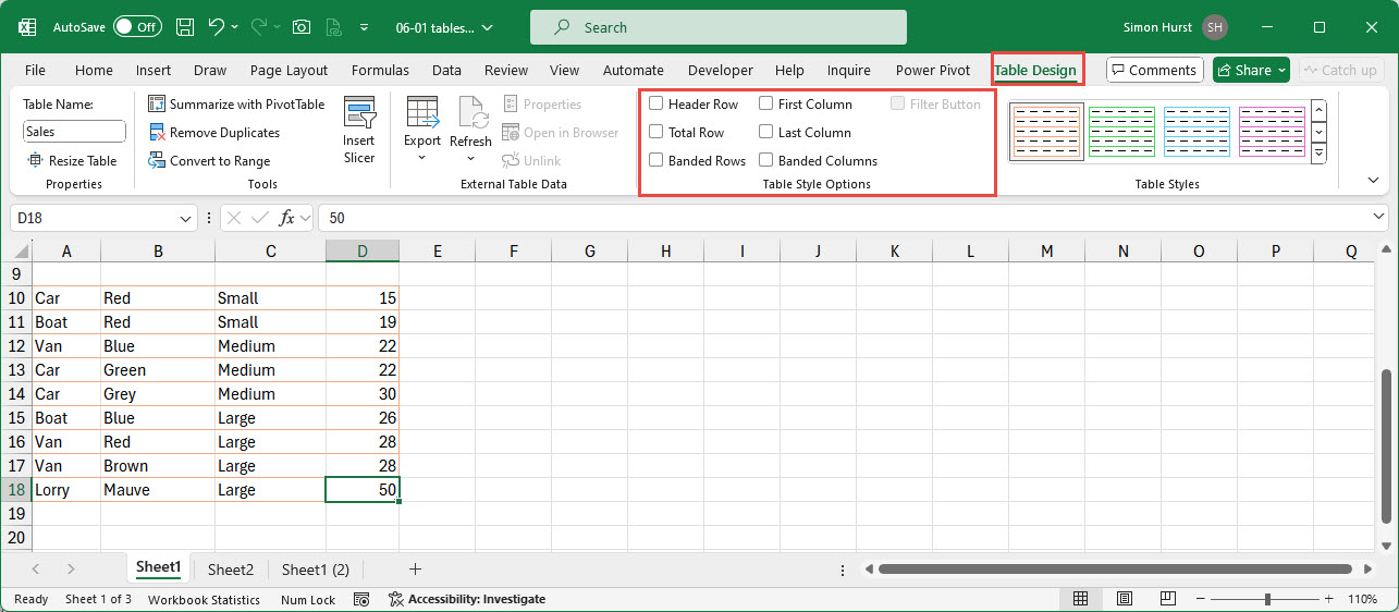
We are going to start by looking at Table Styles. There are two Ribbon tab groups that affect the formatting style applied to the selected Table. Table Style Options and Table Styles.

Here is a four column Table with all of the Table Style Options set to off:

As a comparison, this is the same Table with all of the options turned on:

As you can see, both the Header Row and Total Row can be included or excluded; Rows and Columns can be banded and the First and Last Columns can also be separately emphasised. When the Header row is displayed, it is also possible to turn on or off the Filter Button that displays Filter and Sort options for each column.

The Table Styles group of the ribbon tab displays the Table Styles gallery. Any styles displayed can be applied to the selected Table with a single click, with the dropdown of the gallery displaying all the available styles, arranged by categories Light, Medium and Dark:

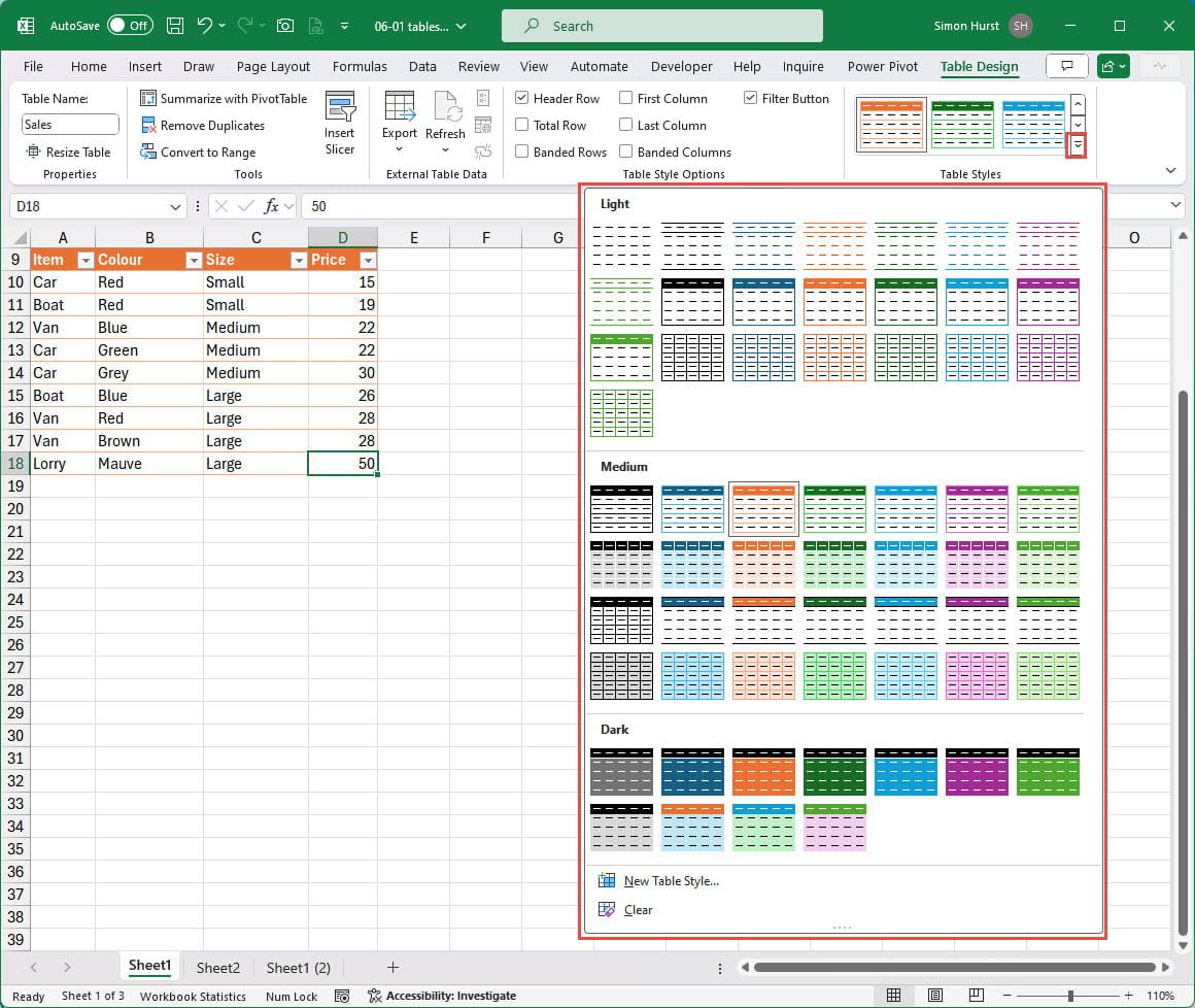
At the bottom of the styles themselves, a Clear button removes all style formatting, and a New Table Style… command allows you to create your own style:

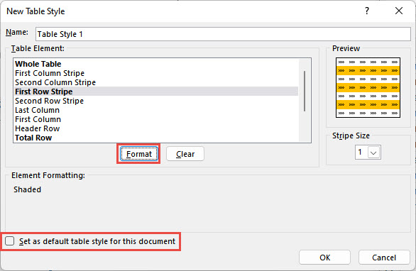
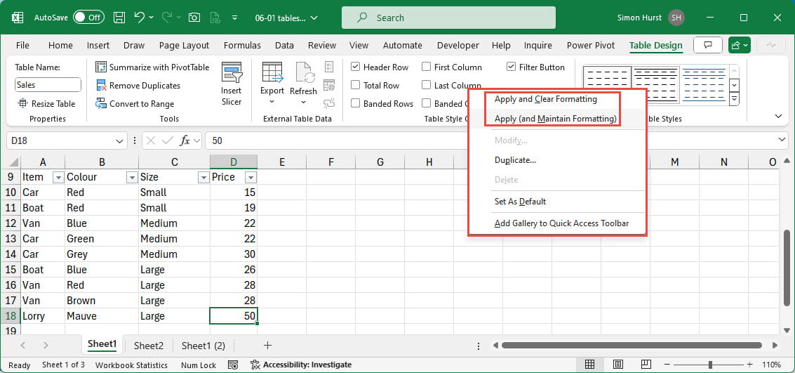
Each Table Element can be formatted using the Format button which displays the Font, Border and Fill tabs of the Format Cells dialog, although the options available from the dialog are limited, depending on the element chosen. It is also possible to set your new table style as the default table style to be used for new tables set up in the same workbook. Existing styles can be set to be the default table style by right-clicking on the style in the style gallery and choosing Set As Default from the right-click menu. This right-click menu also gives some additional control over how a style is applied to an existing table. If you have applied formatting to individual cells in a table, then you can choose whether the style overrides this formatting, or the formatting is maintained:

Custom styles can also be deleted, or modified by displaying the Table Style dialog. Any style can be duplicated to create the basis for a new style.

Table Design Tools

The Table Design Ribbon tab includes a Tools group. This contains four commands. The Summarize with PivotTable command provides one of several ways to create a new PivotTable with the Table as its source. Convert to Range changes the range of cells included in the Table to normal cells that are not part of a Table but does not remove the Table formatting.

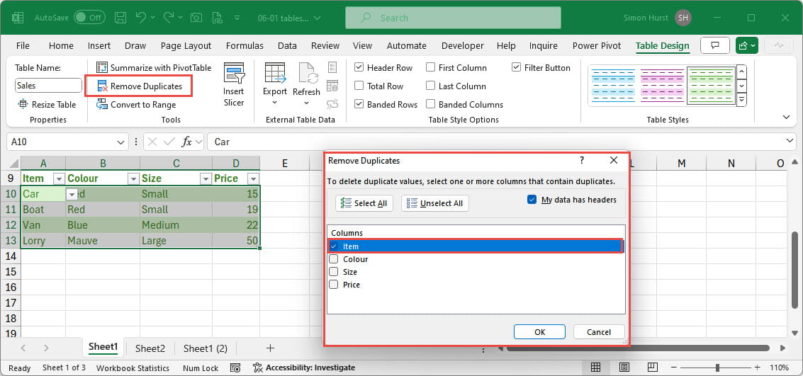
Remove Duplicates provides a way to remove rows that contain duplicated data. Clicking on the command displays a dialog box that allows you to select which columns are used to find duplicated values. For example, if we were just to select the Item column, then we would end up with just the first row for each different value in the Item column in our Table. Where multiple columns are selected, the values in each of the columns must match for the row to be considered as a duplicate:

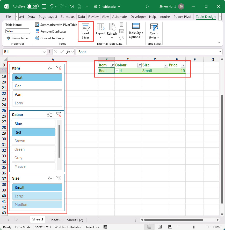
Finally, the Tools group includes the Insert Slicer command. Slicers are visual filters that were first introduced as a way of making PivotTables more interactive. PivotTables support Slicers and a specific type of Slicer, a timeline. Timeline Slicers are not available for a normal Excel Table. Slicers can be added for any Table column and allow only those rows that match all of the Slicer selections to be displayed:

Slicers have their own contextual Ribbon tab and have been covered in other community posts, including their role in using Excel to create interactive dashboards.

Next time…

Next time, we will look in more detail at using Slicers to create a dashboard based on a Table rather than PivotTables.

Conclusion

You can explore Tables, Slicers, dashboards and a great deal more, in the ICAEW archive.