Simple but effective Tables. Part 6 – Dashboards, a refreshing change

Excel Tables – so much more than just a pretty format

When Tables were first introduced into the Windows versions of Excel in Excel 2007, many people saw them as another Excel formatting ‘gimmick’. This view was supported by the inclusion of the Format as Table command in the Styles group of the Excel Home Ribbon tab. However, it soon became apparent that Tables were much more important than that, and that they had a significant role to play in many aspects of automating Excel.

This is the story so far:

• Creating Excel Tables
• The Tables superpower – auto expansion
• Setting Table size manually and the role of Tables in automating Excel
• More automation techniques, including the use of Data Validation and Dynamic Arrays
• The Table Design Ribbon tab options

Having introduced Table Slicers in the previous article, this time we see how to put them to practical use as part of creating an interactive dashboard based on a Table.

Sliced Tables and charts

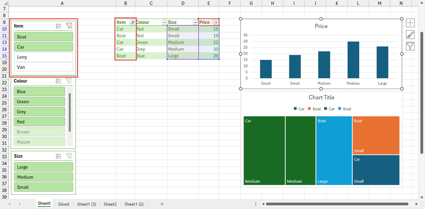
As we saw last time, when we add one or more Slicers based on a Table, selecting one or more items in any of the Slicers will hide any rows in the Table that don’t match all of the Slicer selections. If we base a chart on the whole Table, or on entire columns in the Table, then the chart will also be controlled by the Slicers:

This example demonstrates that our Item Slicer controls the contents of our Table and also the charts that are based on all or part of it. The example also shows an advantage of basing charts on Tables rather than PivotTables. The Treemap style chart cannot be based on a PivotTable, but can be used with a normal Table. However, if we look more closely at our Treemap chart we can see that, for it to work properly, we need to group the items in the range that our chart is based on.

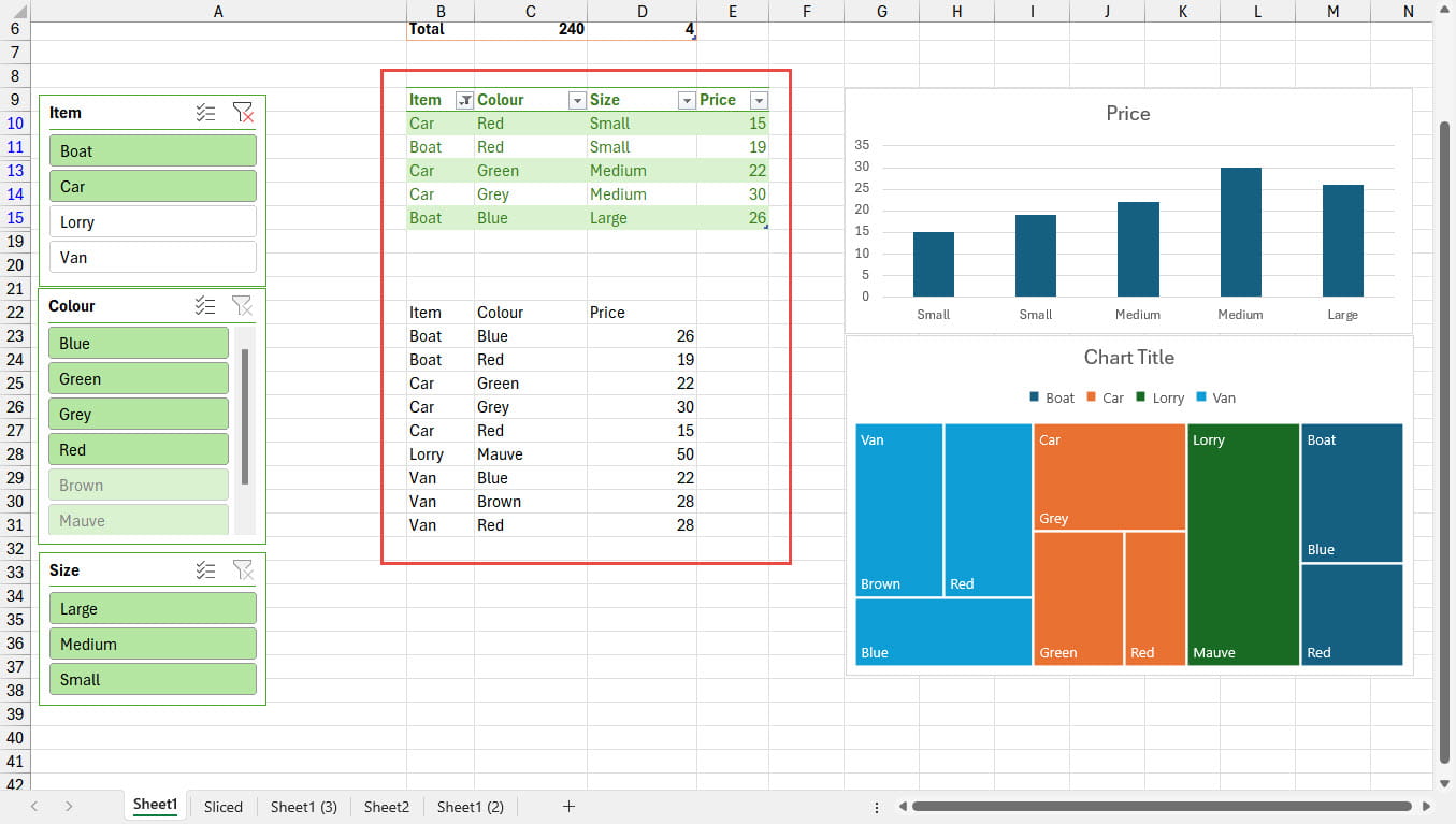
One way of doing this is to use the new GROUPBY() Dynamic Array function that is currently available to those on the Excel ‘Insider’ update channel, and which we looked at very briefly in part 4 of this series. This time we have used a slightly more complicated form of GROUPBY() that groups our Table data by the Item and Colour columns and includes the column headers. Our fourth argument uses the value 3 to include those headers in our output range, with the 0 entered as the fifth argument removing totals from the output:

=GROUPBY(Sales[[#All],[Item]:[Colour]],Sales[[#All],[Price]],SUM,3,0)

Note that we have included our GROUPBY() formula underneath our Table of data for demonstration purposes only, it would usually be preferable to place it elsewhere.

We can base our Treemap chart on our GROUPBY() range but, although it will display the groups in the chart, it will ignore the Slicer settings, since all the rows are still part of the Table that the formula refers to, but are just hidden by the Slicer:

The solution to this is again something that we have covered before. We can add a column to our Table that uses the SUBTOTAL() or AGGREGATE() functions to differentiate between rows that the Slicer has hidden and those that are still displayed.

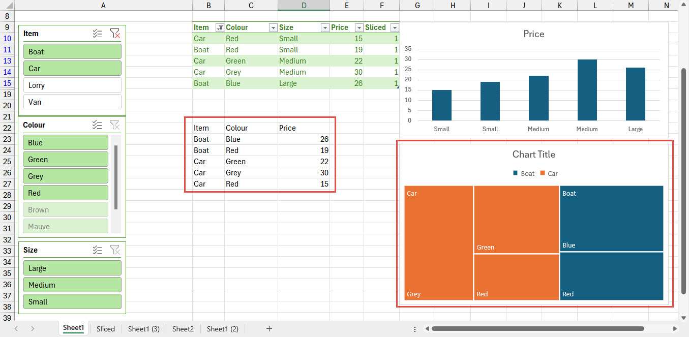
This use of the AGGREGATE() function uses the first argument of 2 to choose the COUNT aggregation, crucially the second is set to 5 to ‘Ignore hidden values’. The array to be aggregated is a single cell. Accordingly, the formula will return a count of 1 for visible rows only:

=AGGREGATE(2,5,[@Price])

By using a function that returns a value such as 1, we can use the column as a filter directly, without needing to compare it to any other value. Here is our ‘Sliced’ column added as the Filter argument of our GROUPBY() function:

=GROUPBY(Sales[[#All],[Item]:[Colour]],Sales[[#All],[Price]],SUM,3,0,,Sales[Sliced])

PIVOTBY() - so near?

You might think that the partner Dynamic Array function to GROUPBY(), PIVOTBY() would mean that we can add other exciting types of chart to our dashboard presentation and thereby avoid the need to use PivotTables, with their need for a refresh operation, entirely. However, there are a few reasons why this might not be the case. Firstly, only simple Slicers can be attached to a Table, whereas there is also a Timeline Slicer available for use with PivotTables. Secondly, Table Slicers can only be attached to a single Table whereas PivotTable Slicers can be connected to multiple PivotTables allowing data from multiple sources to be combined into a single dashboard.

Additionally, there is a problem with the way that PIVOTBY() operates which hopefully might be sorted out before its general release. Because of the way in which it works, PIVOTBY() leaves holes in the output range where any combinations of row and column have no values. This leads to unpredictable results with charts based on PIVOTBY():

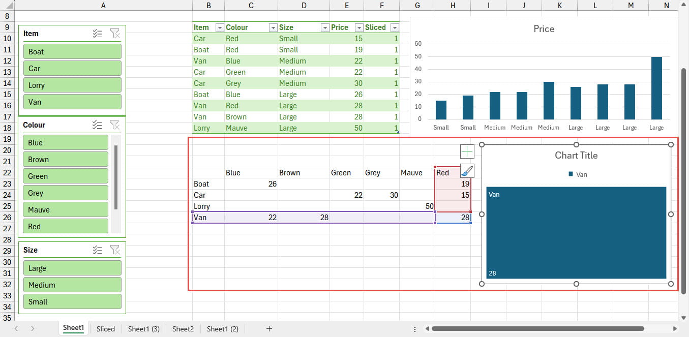
It might look as thought it would be simple enough to replace the blank values with zeros, particularly as the aggregation function used by PIVOTBY() is a LAMBDA() function. Simple as it might be, the solution has eluded me so far. If you know the answer, please let us know via the associated post on in our LinkedIn group:

• ICAEW Excel Community Linkedin Group

Next time…

Next time, we will look at some further Table features and techniques.

Conclusion

You can explore Tables, Slicers, dashboards and a great deal more, in the ICAEW archive.