Simple but effective Tables. Part 8 – Structured References part 2

Excel Tables – so much more than just a pretty format

When Tables were first introduced into the Windows versions of Excel in Excel 2007, many people saw them as another Excel formatting ‘gimmick’. This view was supported by the inclusion of the Format as Table command in the Styles group of the Excel Home Ribbon tab. However, it soon became apparent that Tables were much more important than that, and that they had a significant role to play in many aspects of automating Excel.

This is the story so far:

• Creating Excel Tables
• The Tables superpower – auto expansion
• Setting Table size manually and the role of Tables in automating Excel
• More automation techniques, including the use of Data Validation and Dynamic Arrays
• The Table Design Ribbon tab options
• From Table to Dashboard
• Structured References part 1

Introduction

Several of the previous articles in the series have used ‘structured’ references to refer to Table contents. This is the second of two articles covering structured references. This time we are going to look at structured references within a Table before looking at some more advanced examples of using structured references and seeing how to deal with absolute and relative references.

Structured references within a Table

In the first part of our look at Table structured references we worked with references to Table contents from cells outside of a Table. This time, we’ll look at how structured references work when referring to Table cells from within the same Table. We have adapted our previous example to include a VAT rate column and changed the heading of our existing Amount column to Net. We have also added a Gross column to hold the calculation of the Gross amount. If we create our formula by typing in our formula and clicking on each of the two cells to be used, Excel will create the following formula:

=[@Net]*(1+[@[VAT rate]])

When we accept it, our formula will be copied down to all our other rows:

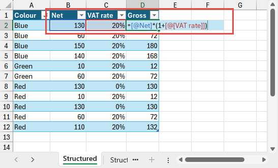
There are two differences from the structured references created from an external cell: there is no need for the reference to include the Table name if it refers to a cell in the same Table, and the @ operator is used to refer to the intersection of the column referenced, with the formula row. Note the difference between single word column header names and header names that include a space. For a single word column header, the @ operator is just added before the column name in a single set of square brackets:

[@Net]

Where there is a space, the column name needs to be included in its own set of brackets with the @ in an additional set:

[@[VAT rate]]

Note that, when Excel Tables were introduced, the ‘this row’ operator was the less concise #This Row before it was replaced by the @ operator.

Other rows

It is also possible to refer to the column header and total rows from within the Table, and to combine such references with ‘this row’ references. Here we have used a reference to the Total of the Gross column to calculate the percentage of each row in the Gross column to the Gross total:

=[@Gross]/Sales[[#Totals],[Gross]]

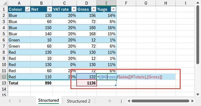
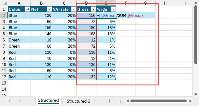
Note that this formula will return a #REF error if the Totals row is switched off. Using the SUM() function with a reference to the entire column might be both simpler and more robust:

=[@Gross]/SUM([Gross])

It’s also worth noting that Table column headers are treated as text so, if you use a number as a column header, referring to that column header using the #Headers operator will return a text value. To use it as a number, you will either need to use the VALUE() function or use a mathematical operator to ‘coerce’ the text value to be treated as a number:

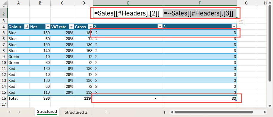
We can see from the column alignment, and the Totals row that a simple reference to the Header of our column 2 returns the text value “2” rather than the number 2, whereas the use of the double minus to coerce our text value of 3 in our column 3 Header converts it to a number.

Referring to multiple columns

It is possible to use the standard : range operator to refer to a contiguous range of columns:

=SUM(Sales[@[2]:[3]])

Absolute and Relative references

By default, references to Table cells or columns, whether in Table cells themselves, or from external cells, are treated as ‘relative’ so if they are copied to other columns they will adjust accordingly:

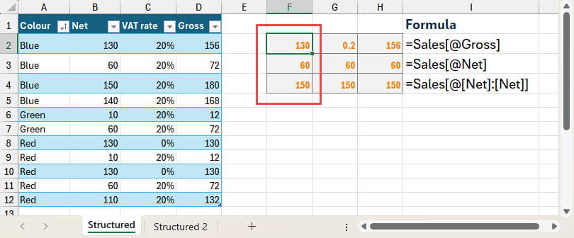
In this example, in column F, we have entered a reference to the cell on the same row in the Net column of our Table. In rows 2 and 3 we have just created a simple reference to the same row in the Net column:

=Sales[@Net]

We have then copied it to columns G and H in two different ways. In row 2 we have used the drag handle. The reference will adjust to create references to the two columns to the right of our Net column, so our formula in column H will end up as:

=Sales[@Gross]

In row 3, we have selected our three cells and used the Control+r keyboard shortcut to ‘fill right’. This copies the reference without making it relative, so creates the same reference in each cell:

=Sales[@Net]

Although these two methods can help us cope when we just need all relative, or all absolute references, they will not allow us to copy a formula correctly that contains a reference that we want to treat as relative, and another that we want to treat as absolute. To cope with this, we can force a column reference to be treated as absolute by using a range of columns. The range being one column to the same column:

=Sales[@[Net]:[Net]]

The syntax for this reference is not straightforward, so the easiest way to create it could be to create a reference to a range of two columns and then edit the formula to replace the header name in one of those references:

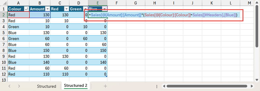
Here is an example that combines most of the techniques we have covered this time. We have added columns to our Table to allow us to create separate columns for our three Colour values. We want to be able to enter a single formula in column C and then copy it to columns D and E. We fix our references to the Amount and Colour columns by using a range that refers to a single column in each case. The reference to the Colour in the header of each of our columns needs to be relative so this is just entered as a simple reference to the current column header so it will adjust when copied across:

=Sales[@[Amount]:[Amount]]*(Sales[@[Colour]:[Colour]]=Sales[[#Headers],[Blue]])

Next time…

Next time, we will look at some of the less obvious capabilities of Excel Tables.

Conclusion

You can explore all aspects of Tables, and a great deal more, in the ICAEW archive.