Simple but effective Tables: Part 9 – sorting, filtering, Sparklines and check boxes

Excel Tables – so much more than just a pretty format

When Tables were first introduced into the Windows versions of Excel in Excel 2007, many people saw them as another Excel formatting ‘gimmick’. This view was supported by the inclusion of the Format as Table command in the Styles group of the Excel Home Ribbon tab. However, it soon became apparent that Tables were much more important than that, and that they had a significant role to play in many aspects of automating Excel.

This is the story so far:

• Creating Excel Tables
• The Tables superpower – auto expansion
• Setting Table size manually and the role of Tables in automating Excel
• More automation techniques, including the use of Data Validation and Dynamic Arrays
• The Table Design Ribbon tab options
• From Table to Dashboard
• Structured References part 1
• Structured References part 2

Introduction

Having covered the more obvious features of Excel Tables over the previous 8 parts of the series, we will finish the series by looking at some of the other features that we haven’t yet covered.

Sorting and Filtering

The ability to sort and filter a column is not restricted to columns in Tables but, unlike a column outside of a Table, filter buttons are included by default in the header row of a Table. These buttons can be toggled on or off using the Filter Button checkbox in the Table Style Options group of the Table Design Ribbon tab. The filter and sort options available in the Filter Button dropdown in each Table column heading depend on the contents of that column and include a list of the different values in the column, allowing a value to be selected with a single click. As well as values, filter and sort options also include some format properties such as font colour and cell fill colour. One of the properties that can automatically be copied down to new Table rows is consistent conditional formatting. Some conditional formats can be used for sorting and filtering. Conditional formatting Colour Scales change the cell fill colour and the different colours used as part of the scale will show up in the Sort by Colour and Filter by Colour menus. Perhaps more surprisingly, conditional formatting icons will also be available:

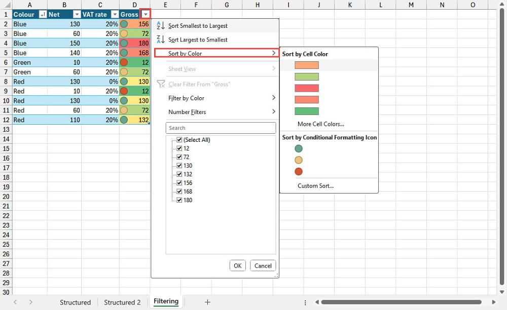
Note that at the bottom of the Sort by Colour menu there is a Custom option that will allow you to sort by multiple levels including using different columns and choosing cell values, cell colours, fill colours or conditional formatting icons. The sort order for each level can be swapped between Smallest to Largest, Largest to Smallest for value columns, and A-Z, Z-A for text columns. It is also possible to sort either type of column using a Custom List which can be useful for values such as months or days of the week for example.

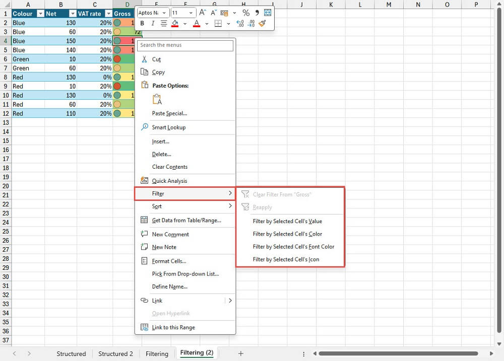
Sorts or filters can also be applied by right-clicking on a particular cell in a Table, or in a non-Table cell. The right-click menu includes Filter and Sort options with general options to Sort, or to Clear or Reapply a filter, as well as Sort and Filter options relating to the specific cell contents:

Although the Filter options covered so far are not exclusively available in Tables, the use of the more visual ‘Slicer’ filter is limited to Tables and PivotTables. There is also a specific ‘Timeline slicer’ for filtering columns that contain data or time values, but this is not available in Tables. Another feature of Slicers that is restricted to PivotTables is the ability to connect a Slicer to multiple PivotTables. A Table Slicer only works on a single Table. In part 5 of the series, we saw how to use the Insert Slicer command in the Table Design Ribbon tab to add a Slicer to a Table.

Extending columns – it’s not just formulas

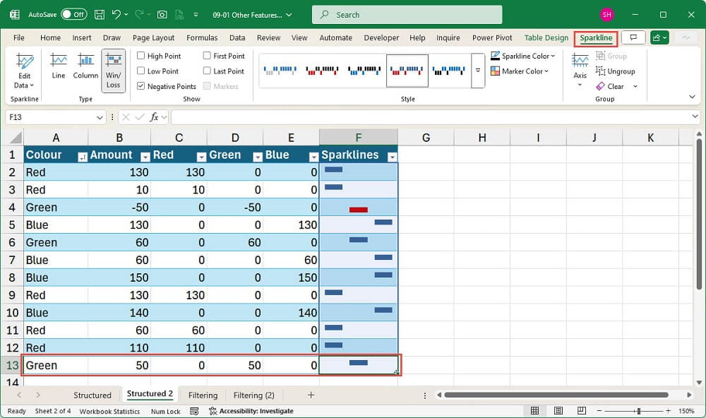
One of the first Table capabilities that we covered in this series was the automatic copying of formulas down to new rows as they are added to the Table. It’s not just the copying of formulas that can be automated in this way. If you insert Sparklines in a Table column, then the Sparklines will be copied to new rows:

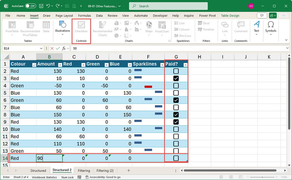
A recent enhancement now allows check boxes to be added directly to cells. If check boxes are inserted into a Table column, just like Sparklines, a check box will automatically be added to new rows as they are added to the column:

Next time…

Next time, we will look at some issues and opportunities around the worksheet Tables created by Power Query.

Conclusion

• You can explore all aspects of Tables, and a great deal more, in the ICAEW archive