Simple but effective Tables. Part 7 – Structured References part 1

Excel Tables – so much more than just a pretty format

When Tables were first introduced into the Windows versions of Excel in Excel 2007, many people saw them as another Excel formatting ‘gimmick’. This view was supported by the inclusion of the Format as Table command in the Styles group of the Excel Home Ribbon tab. However, it soon became apparent that Tables were much more important than that, and that they had a significant role to play in many aspects of automating Excel.

This is the story so far:

• Creating Excel Tables
• The Tables superpower – auto expansion
• Setting Table size manually and the role of Tables in automating Excel
• More automation techniques, including the use of Data Validation and Dynamic Arrays
• The Table Design Ribbon tab options
• From Table to Dashboard

Introduction

Several of the previous articles in the series have used ‘structured’ references to refer to Table contents. This is the first of two articles covering structured references. This time we are going to look in more detail at how structured references work when used outside of a Table. We will first see how to create them, before moving on next time to investigate their use within Tables and also some more advanced structured references.

Creating structured references

Perhaps the easiest way to create a structured reference is just to drag across the cells in the same way that you would to create any reference to a range of cells. In this example we have created a small Excel Table and used the Table Design Ribbon tab, Properties group, Table Name: box to give it the descriptive name: Sales.

In cell H2 we have entered a SUM() function by using the Alt+= keyboard shortcut and then dragged across a range of cells from B2 down to B12:

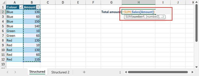
Because our range is an entire Table column, Excel will replace the normal cell coordinate reference with the name of the Table, followed by the column heading. This gives us a much more informative formula than a cell range of B2:B12:

=SUM(Sales[Amount])

If you are really unconvinced about the benefits of using structured references when referring to Table contents, there is an Excel option to turn the behaviour off. In the File, Options dialog, the Formulas category includes a ‘Working with formulas’ section that has an Option to turn off ‘Use table names in formulas’. With this option turned off, dragging down an entire Table column will create a ‘normal’ range reference:

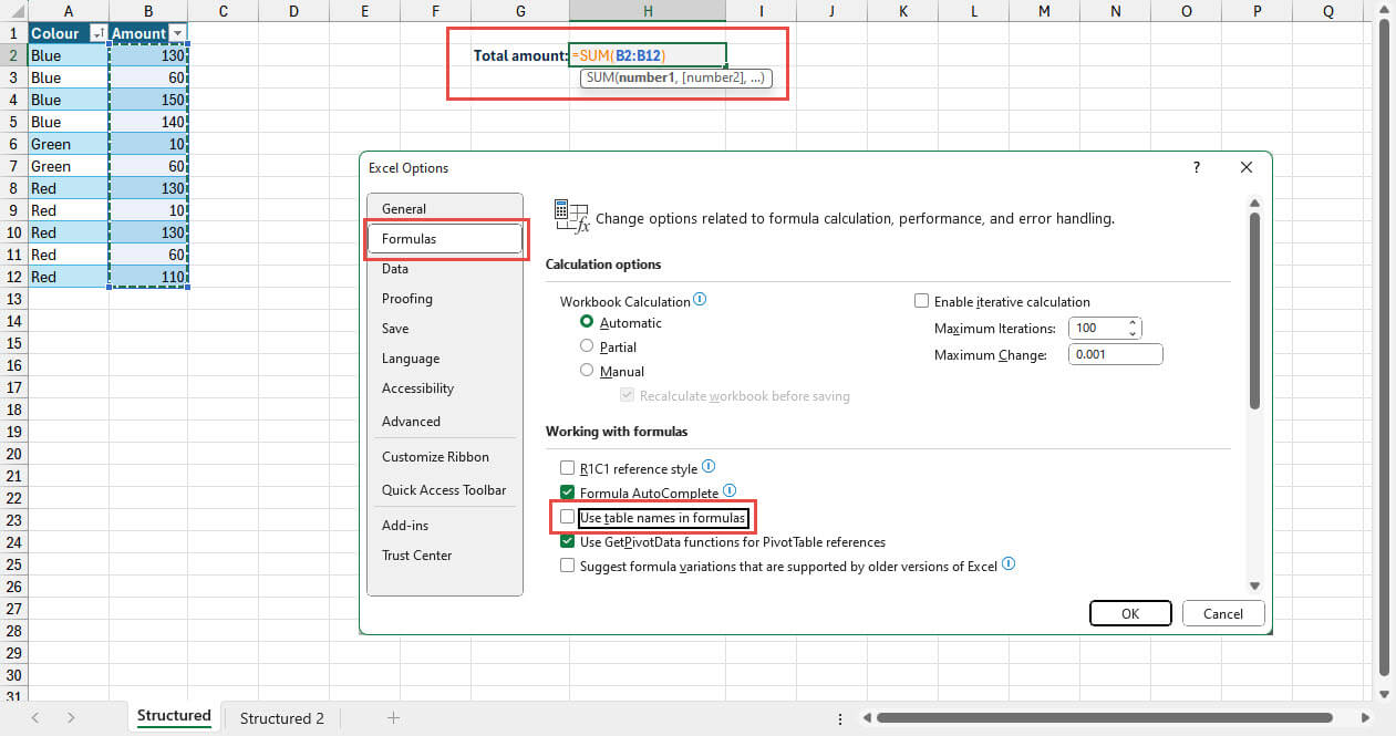
Given that this article is all about using structured references, we will turn the option back on before continuing.

Because our total cell is near to our Table, it’s easy to create our range reference by dragging. If we wanted to refer to our Table contents from a different sheet, it would be slightly less straightforward. We would need to know which sheet our Table was located on and then switch to that sheet before we could drag over the relevant cells. In these circumstances, it can be easier to let Excel’s AutoComplete feature do the work. If we know the name of our Table, we can start typing the name and Excel will display matches in the AutoComplete list:

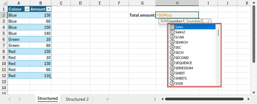
We can see that, having just typed in the letter ‘s’, our Sales Table appears at the top of the alphabetical list of AutoComplete objects, with the icon helping to distinguish the Tables from the functions in the list. We can double-click on Sales, or use the keyboard Tab key to accept the current selection, to start our range reference. We just want to total a single column so, once we have entered our ‘Sales’ reference, we use the keyboard left square bracket to display the next step of our AutoComplete list. This includes our column names which we can include using the Tab key or double-click as before:

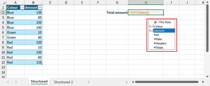
We can then finish our reference with our right square bracket:

=SUM(Sales[Amount])

Modifiers

As you can see from the AutoComplete list above, there are more options available than just our Table columns. It is possible to modify our reference to just refer to the current row using the @ sign. This requires the formula to be on the same row as one of our Table rows, or the formula will return a #VALUE! error.

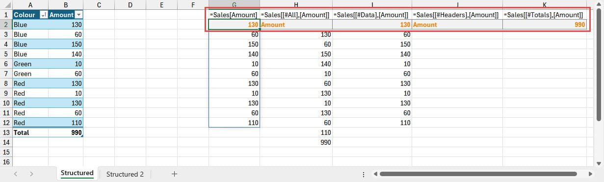
There are four other modifiers available that specify which part of the Table or Table column to include in the reference. By default, a reference will just refer to the Data area of the Table – the rows between the Header row and the Total Row. However, the modifiers allow us to specify the Data area explicitly, as well as to specify the whole column or table as well as the Header row and the Totals row. Here we have used Dynamic Arrays to demonstrate the use of the different options and to show that #DATA returns the same range as omitting the modifier:

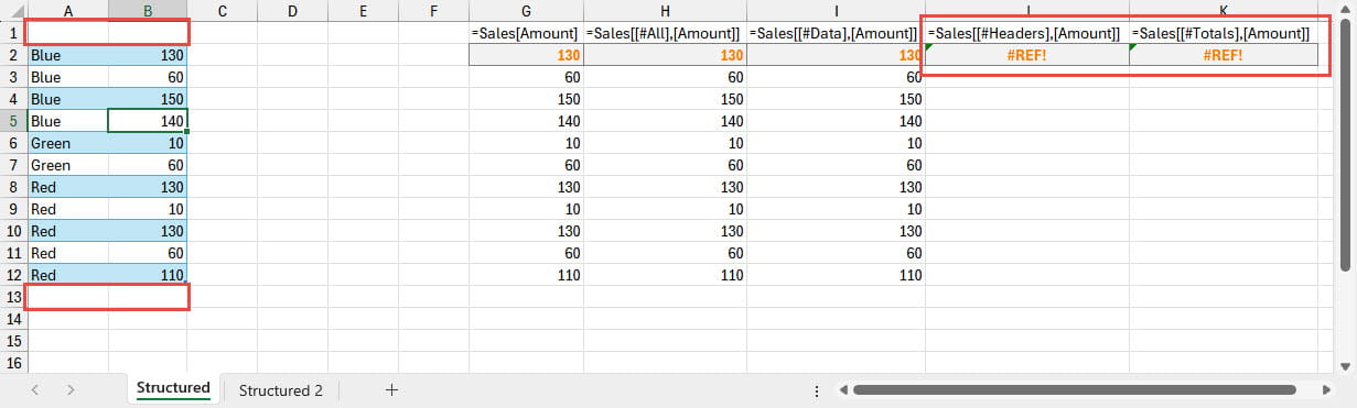
Note that if the Table Design Ribbon tab options are set to suppress the Header and or Totals row, the formulas that include the specific modifier will return an error:

The easiest way to include modifiers in structured references is just to drag over the required range. If you want to use AutoComplete to include modifiers, then note that, after entering or selecting the Table name, it is necessary to type two, rather than one, left square brackets before choosing the modifier from the AutoComplete list. After the modifier and a right square bracket, entering a comma, followed by another left square bracket, will display the AutoComplete list again to enter the Column name, with two right square brackets required at the end of the range:

=Sales[[#All],[Amount]]

Total double trouble

It’s also worth noting that, were you to use an aggregate function in the Totals row, and to use the #ALL modifier, the resulting value will depend on whether or not the Totals row is suppressed. With the display of the Totals row turned on, the formula result would include any aggregate value selected in the Totals row for that column, potentially causing an error. For example, if the Totals row for that column was set to SUM, then a SUM() formula, with the #ALL modifier as part of the reference, would return the sum of the individual items plus the total itself, so doubling the resulting value.

It would be quite easy to create this problem inadvertently. If the Totals row was turned on, and an aggregate function chosen for the column before the Totals row was suppressed again, then dragging a range that included the Header, as well as the Data area, would use the #ALL modifier. Although the formula might give the correct result initially, as soon as the Totals row was turned on again, the range would include the individual rows as well as the Totals row aggregate value.

Next time…

Next time, we will look at structured references within Tables, references that include multiple columns and how to deal with absolute and relative references to Table columns.

Conclusion

You can explore all aspects of Tables, and a great deal more, in the ICAEW archive.