With Excel’s dynamic array calculation engine, we can do some amazing things. It opens up solutions which were previously impossible.

However, one area that causes issues is how Excel handles an array of arrays.

What is an array of arrays?

Excel’s calculation engine spills results into multiple cells; and it can do this in a variety of ways.

Let’s look at XLOOKUP as an example.

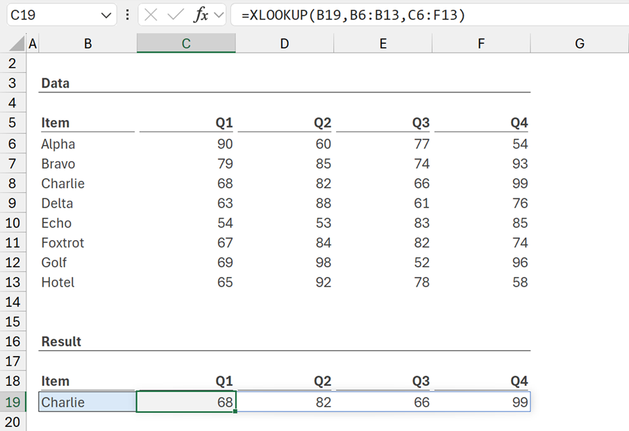
The formula in cell C19 is:

=XLOOKUP(B19,B6:B13,C6:F13)

This formula looks up Charlie from B6:B13 and returns all the corresponding columns from the range C6:F13.

Since the formula returns 4 columns (columns C:F), Excel spills the 4 values into cells C19:F19.

This demonstrates that from one lookup value, Excel can return multiple columns.

Now let’s look at another way in which XLOOKUP spills.

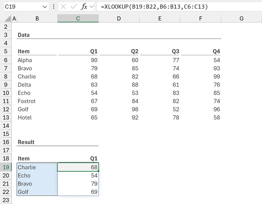
The formula in cell C19 is:

=XLOOKUP(B19:B22,B6:B13,C6:C13)

This formula is looking up Charlie, Echo, Bravo and Golf from B6:B13 and returning the range from a single column C6:C13.

XLOOKUP expects a single lookup value. However, if it receives multiple values, it performs the XLOOKUP calculation for each value and returns the result for all of them as an array (this is known as lifting).

Therefore, in the example above XLOOKUP calculates 4 times, once for each lookup value.

This demonstrates that from multiple lookup values, Excel can return a single column.

So far so good. The issue comes when we combine these methods.

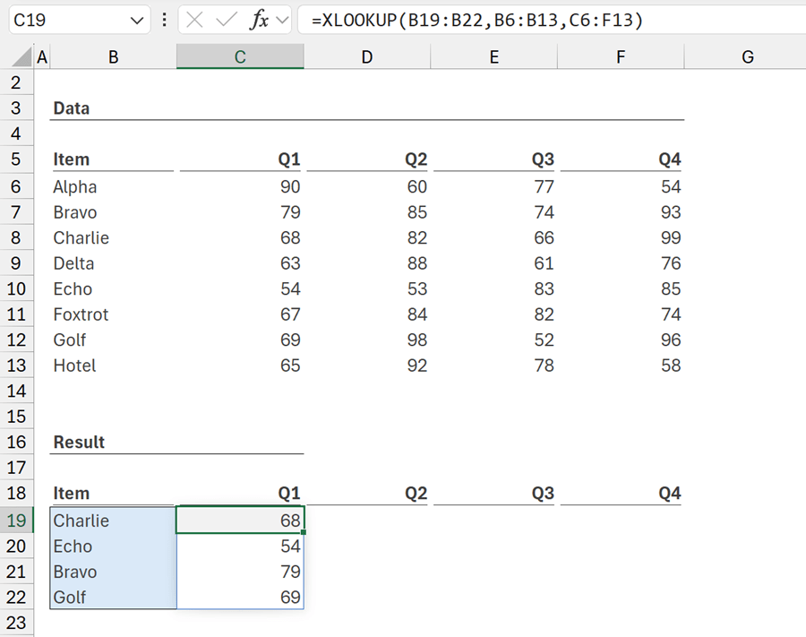
The formula in cell C19 is:

=XLOOKUP(B19:B22,B6:B13,C6:F13)

This formula is looking up Charlie, Echo, Bravo and Golf from B6:B13 and is trying to return all the columns from C6:F13. However, it doesn’t work. It only returns the first result.

Surely, if there are multiple columns in the return array, we should get the values spilling across the columns?

Unfortunately, not. This is caused by the array of arrays issue.

XLOOKUP calculates once for each lookup value.  However, the return array of each calculation is not a value, but an array. Therefore, the function is not creating a 2-dimensional array of values, but an array of arrays.

How to resolve the array of arrays issue?

You’re probably thinking. “OK, so how do we resolve the array of arrays issue?”

The answer is: We can’t. That’s just how Excel works.

However, that doesn’t mean we can’t build formulas in different ways and therefore avoid the issue entirely.

For any given scenario, we may be able to create a specific formula to calculate the expected result without creating an array of arrays.

For the XLOOKUP example above, we could use the following:

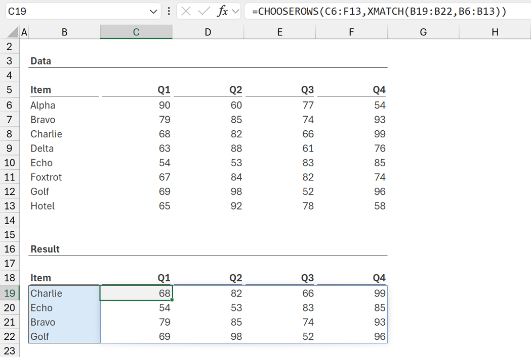
The formula in cell C19 is:

=CHOOSEROWS(C6:F13,XMATCH(B19:B22,B6:B13))

With this formula, the values spill into the rows and columns, which is exactly the result we want.

This formula works in this specific situation, but not all array of array situations. So, this requires us to think through different solutions to find one that works for our exact scenario.

However, there is also a more generic solution which works in many array of array scenarios. It uses a DROP, REDUCE, LAMBDA, VSTACK/HSTACK combination.

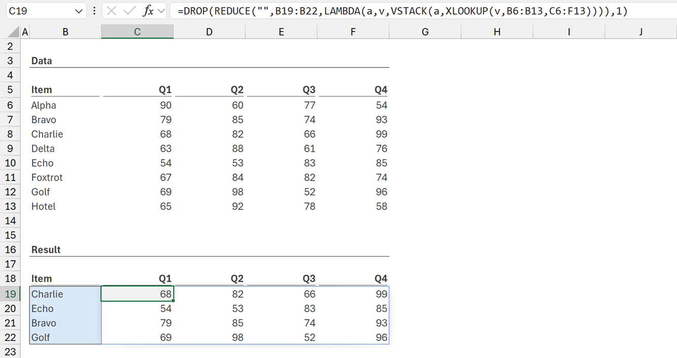
The formula in cell C19 is:

=DROP(REDUCE("",B19:B22,LAMBDA(a,v,VSTACK(a,XLOOKUP(v,B6:B13,C6:F13)))),1)

Using this formula, we calculate the result without the array of arrays problem.

Effectively, it loops through each cell in B19:B22 and calculates the XLOOKUP for each of those cells. The result of each XLOOKUP stacks together into a single result.

This DROP, REDUCE, LAMBDA, HSTACK/VSTACK combination is a common pattern for advanced Excel formulas.

We will look in more detail at this combination in a future post.

Applying the pattern

Let’s take a look at another example.

In TEXTSPLIT, if we have a single cell, Excel will happily spill the result.

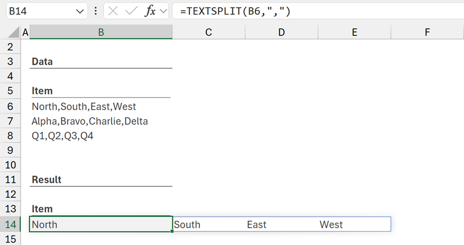
The formula in cell B14 is:

=TEXTSPLIT(B6,",")

Using the comma as a delimiter, the formula spills the text in cell B6 across multiple columns.

If we try to perform this calculation across many rows we get the array of arrays issue again.

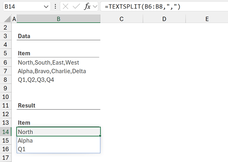
The formula in cell B14 is:

=TEXTSPLIT(B6:B8,",")

We are trying to split the values in the range B6:B8. Rather than spilling the results across rows and columns, it only returns the first value.

There are various specific formulas we could use as a solution. But we also have the DROP, REDUCE, LAMBDA, VSTACK/HSTACK pattern we can use.

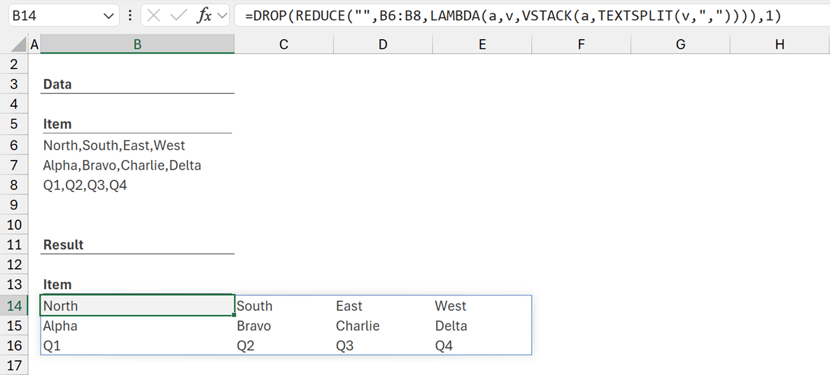
The formula in cell B14 is:

=DROP(REDUCE("",B6:B8,LAMBDA(a,v,VSTACK(a,TEXTSPLIT(v,",")))),1)

This spills the result as we would expect.

Let’s compare this to the XLOOKUP solution from earlier:

TEXTSPLIT:

=DROP(REDUCE("",B6:B8,LAMBDA(a,v,VSTACK(a,TEXTSPLIT(v,",")))),1)

XLOOKUP:

=DROP(REDUCE("",B19:B22,LAMBDA(a,v,VSTACK(a,XLOOKUP(v,B6:B13,C6:F13)))),1)

The only sections which differ is the range to loop over and the specific function to use. So, we have applied the same pattern in both scenarios.

Working with arrays of different sizes

What happens if our arrays are not all the same size?

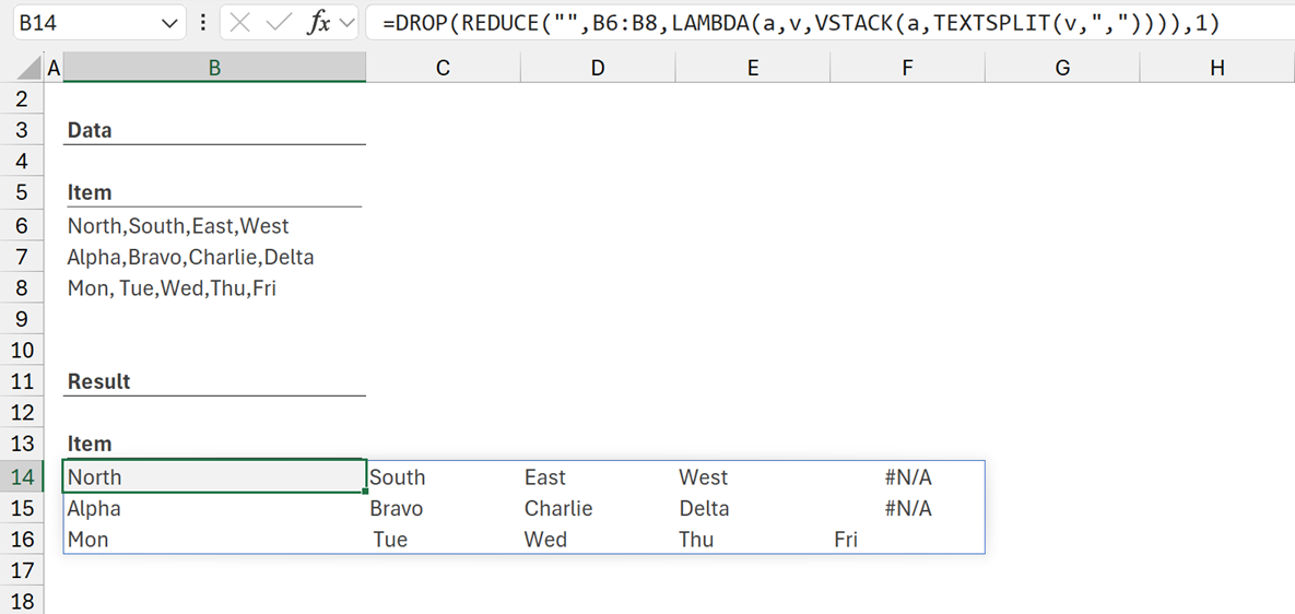
In this example, we changed the value in cell B8, Q1, Q2, Q3, Q4 (an array with 4 items) to Mon, Tue, Wed, Thu, Fri (an array with 5 items). Therefore, the individual rows no longer contain the same number of items. Excel padded the shorter arrays with #N/A to ensure they were the same size.

It's unlikely we want #N/A in our result. So, we can wrap IFERROR around the result to display alternative values.

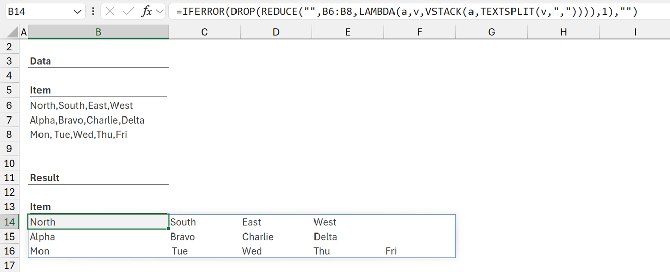
The formula in cell B14 is:

=IFERROR(DROP(REDUCE("",B6:B8,LAMBDA(a,v,VSTACK(a,TEXTSPLIT(v,",")))),1),"")

In this formula, we replaced #N/A with an empty text string.

Notes

Before we wrap up, there are a few things to be aware of:

Speed

While this pattern is powerful, recalculation can be slow. Therefore, in some situations we may want to look for alternative specific solutions which are faster.

However, the DROP, REDUCE, LAMBDA, HSTACK/VSTACK combination will provide a suitable solution in many scenarios.

Orientation

In the examples above, we used VSTACK because the calculation in each row spills horizontally. Therefore, we needed to stack the results vertically.

Therefore, if we have a calculation which spills vertically, we will need to use the HSTACK function instead of VSTACK.

Conclusion

The array of arrays issue can be difficult to understand and problematic to resolve.

While we can create specific solutions, in this post, we have seen there is a generic solution which will work in many array of array scenarios.