Introduction

Yes, it’s that time of year again. The time of year when a normally decent pub quiz feels the necessity to swap questions on tropical hardwood varieties for exclusively festive-themed brainteasers. That being the case, it’s almost inevitable that you are about to be asked to calculate the total number of presents gifted during the 12 days of Christmas. In the unlikely event that you have forgotten the correct answer since this time last year, we thought we’d use the calculation to demonstrate some of the capabilities of the LAMBDA() helper functions as an alternative to working out the solution algebraically.

MAKEARRAY()

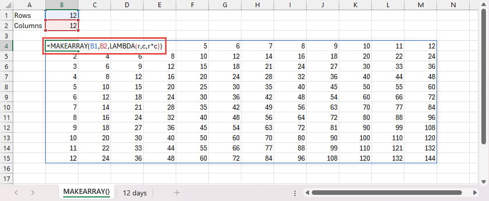
Let’s start with the MAKEARRAY() function. This creates an array by taking the row and column index numbers and using them in a LAMBDA() calculation. For example, you could generate a set of ‘times tables’ by setting the number of rows and number of columns both to 12 and then setting the calculation to be row * column. So, for row one of the array, the row number will be 1 and the column numbers will be 1-12; for row two, the row number will be 2 and the column numbers will still be 1-12. Multiplying the row number by the column number will generate the 2 times table in row 2 and so on for the 12 rows of the array:

=MAKEARRAY(B1,B2,LAMBDA(r,c,r*c))

We have entered our number of rows in cell B1 and referred to that cell as the first argument of MAKEARRAY() to generate 12 rows. Our second argument refers to cell B2 to generate 12 columns. We then use a LAMBDA() function where we pass through the row number (r) and column number (c) to our calculation r*c:

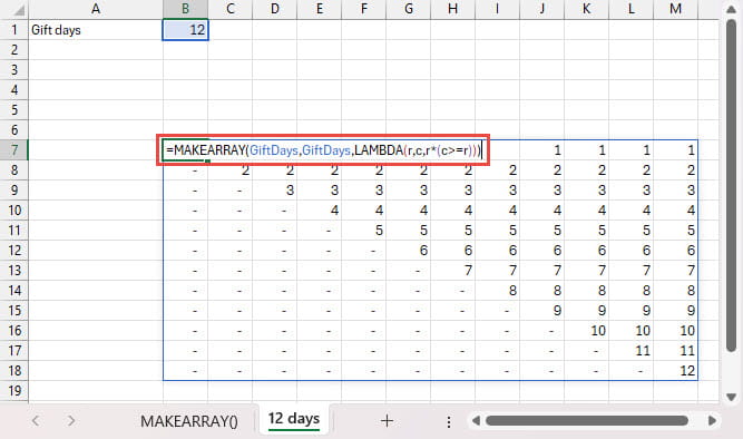
Our next task is to come up with a calculation that matches our Christmas gifting plan. Our rows will represent the number of presents, and the columns the days of Christmas. For our first column, we only want a value in row 1, for our second column – the second day of Christmas – we just want the values in row 1 and row 2, and so on through our 12 days. Our calculation needs to use the column number to exclude the row values, so we set our calculation to be the row number multiplied by whether the column number is greater than, or equal, to the row number:

r*(c>=r)

The Boolean values returned by comparisons are 1 for TRUE and 0 for FALSE. Where our row, column comparison is TRUE we will return our row number, where it is FALSE we will return zero.

Using row two as an example, in row 2, column 1, the calculation will be:

2*(1>=2) = 2*FALSE = 2*0 = 0

In row 2, column 2, the calculation will be:

2*(2>=2) = 2*TRUE = 2*1 = 2

For all the remaining columns, the column number will be greater than the row number so our comparison will generate TRUE and our row number of 2 will be included. As we go down our rows, the pattern will be repeated to create our number of gifts by day:

=MAKEARRAY(GiftDays,GiftDays,LAMBDA(r,c,r*(c>=r)))

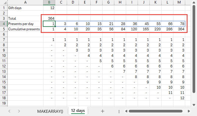
One of the most useful aspects of working with Dynamic Array functions is that you can see the result of your calculation rather than it being hidden in the black box of a function calculation. Of course, if you just want to know the answer, it would be useful to be able to add up all of our 144 individual values and show the result in a single cell. We can do this using another LAMBDA() helper function: REDUCE(). This function reduces an array to a single value by applying an aggregate calculation to each item in the array. We can use our MAKEARRAY() formula as the array argument in REDUCE():

=REDUCE(0,MAKEARRAY(GiftDays,GiftDays,LAMBDA(r,c,r*(c>=r))),LAMBDA(a,b,SUM(a+b)))

The calculation in REDUCE() uses a LAMBDA() function with two parameters, the first acts as an accumulator that starts with the value specified in the first argument of the REDUCE() function. The second argument is a variable that represents each of the individual values in our array. So, our calculation adds each item in our array to an initial value of 0 to accumulate the sum of all of our values. This all looks rather complicated, but fortunately it is possible to simplify the second LAMBDA() to just the aggregate function that it uses:

=REDUCE(0,MAKEARRAY(GiftDays,GiftDays,LAMBDA(r,c,r*(c>=r))),SUM)

Having mastered these techniques, you can go on to using BYCOL() to calculate the number of gifts per day:

=BYCOL(MAKEARRAY(GiftDays,GiftDays,LAMBDA(r,c,r*(c>=r))),SUM)

and SCAN() to calculate the cumulative number of gifts given by the end of each day:

=SCAN(0,BYCOL(MAKEARRAY(GiftDays,GiftDays,LAMBDA(r,c,r*(c>=r))),SUM),SUM)

You can explore all aspects of Excel, including other Christmas special series, in the ICAEW archive:

• Excel archive