The new GROUPBY() and PIVOTBY() functions have recently been added to the production editions of Excel. We have already included several articles covering the use of the new functions, including:

• Using slicers with PIVOTBY, GROUPBY and FILTER

• Excel's new functions might change data analysis forever

In this post, we are just going to have a look at one additional capability of both of the two new functions: the ability to use other functions and formulas within the individual arguments of each function.

Grouping by part of a field

In this example, each of our product codes is a composite value with three components, separated by dashes:

GUA-NOR-24

We are assuming that we need to group our data using just one of those components. For example, the first three characters might represent a category of product. To group our product rows by this category using the GROUPBY() function, we could include the LEFT() function as part of our first ’row_fields’ argument.

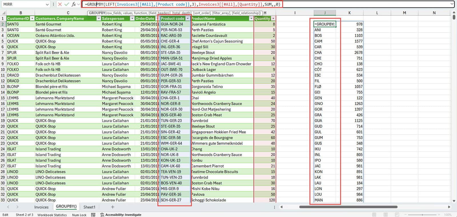
Here we are grouping by the first three characters of our Product code field:

=GROUPBY(LEFT(Invoices3[[#All],[Product code]],3),Invoices3[[#All],[Quantity]],SUM,,0)

In this example, we have used the [#All] modifier to include our Table header row, as well as all of the data values in the Product code column. The fourth argument of our GROUPBY() function allows us to include that header in our resulting table, but doing so does reveal an issue with applying a formula to our column:

As we can see, our LEFT() function is not only applied to our data values, but also to the header value, converting Product code into ‘Pro’. For this reason, if you are working with fixed columns, you might find it better to leave the automatic headers out and instead type them in manually.

Let’s go a bit further and use the same field from the original Table of data to create two groups. We are going to use the MID() function to group by 3 characters starting at position 5 (one position after our first three characters and the delimiter). In order to create two groups, we are going to wrap our two text functions within the HSTACK() function. This Dynamic Array function combines 2 or more arrays into multiple columns. We have also changed our Table column references to just use the data rows by removing the [#ALL] modifiers from each of our ranges. We have replaced the automatically generated headers with text:

=GROUPBY(HSTACK(LEFT(Invoices3[Product code],3),MID(Invoices3[Product code],5,3)),Invoices3[Quantity],SUM,,0)

Grouping row and column fields in PIVOTBY()

The same techniques would also work with the PIVOTBY() function. Here, we have used our previous, HSTACK(), example to generate our ‘row_fields’, and then used the YEAR() function with our OrderDate field to create the group for our ‘col_fields’ argument. We have also deleted the manual headers from the previous example:

Additional resources

You can explore all aspects of Excel, including many articles on conditional formatting, in the ICAEW archive.