FILTER has fast become one of the most useful functions in Excel. It is flexible and simple to use.

In our recent ‘Excel Tips & Tricks Live – your questions answered’ webinar, we touched on how the function can be used to filter large amounts of data. In this post we delve deeper into just one argument to discover new ways for using FILTER in advanced scenarios.

The truth about FILTER

Let’s start with a brief recap of the FILTER function.

FILTER syntax and arguments

FILTER has 3 arguments:

Syntax:

=FILTER(array, include, [if_empty])

Arguments:

• Array: The range of cells, or array of values to filter.
• Include: An array of TRUE/FALSE results, where the TRUE values are retained in the filter.
• [if_empty]: The value to display if no rows are returned. Optional.

Simple Example

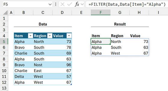
The formula in cell F5 is:

=FILTER(Data,Data[Item]="Alpha")

The formula returns the values from the table called Data, where the elements in the Item column are equal to Alpha.

We can create AND logic using multiplication between multiple conditions.

For example, to return the rows where Item is equal to Alpha and Region is equal to North, we would use:

=FILTER(Data,(Data[Item]="Alpha")*(Data[Region]="North"))

Brackets are required around each condition to ensure calculation occurs in the right order.

To create an OR condition, we use addition between conditions. For example, to return the rows where Item is equal to Alpha or Item is equal to, Charlie we use:

=FILTER(Data,(Data[Item]="Alpha")+(Data[Item]="Charlie"))

We can mix and match OR and AND conditions, using brackets as required to achieve the correct calculation order.

Include argument

It’s easy to think, the include argument must contain a condition, where the matching items are returned. However, it’s simpler than this. FILTER merely requires a TRUE or FALSE result for each element in the array. Any element with a corresponding TRUE is included in the result, and any element corresponding to FALSE is excluded.

Therefore, to push FILTER to new heights, we simply need to think of useful ways to create TRUE or FALSE results for each row. That’s what we are looking at for the remainder of this post.

Note: Excel treats any non-zero number as TRUE and zero as FALSE.

Return alternating rows

Using the SEQUENCE and MOD functions we can create a sequence of numbers which allow us to return alternating rows.

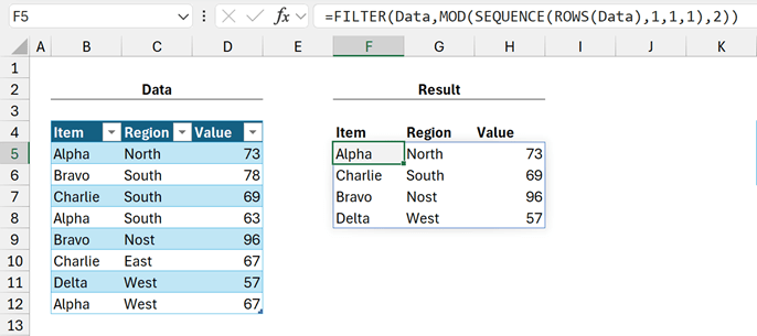
The formula in cell F5 is:

=FILTER(Data,MOD(SEQUENCE(ROWS(Data),1,1,1),2))

• ROWS counts the number of rows in the Table: 8
• SEQUENCE creates a list of numbers based on the row count: {1;2;3;4;5;6;7;8}
• MOD(x,2) converts the sequence into an arrayof 1’s (TRUE) and 0’s (FALSE): {1;0;1;0;1;0;1;0}

Applying this inside FILTER returns the alternating rows from the data.

Changing the divisor argument inside MOD, or the start and step values inside SEQUENCE, provide different patterns for returning values.

Wildcard search

The FILTER function does not allow for wildcard searches. However, we can make use of SEARCH to perform a partial text match.

SEARCH returns the character position at which a specified text string starts.

Let’s look at the following example:

=SEARCH("Excel","ICAEW Excel Community")

The word Excel starts at the 7^th character within ICAEW Excel Community. So, the function returns 7.

In the following formula, there is no matching text.

=SEARCH("Google Sheets","ICAEW Excel Community")

As there is no match, the result of this function is the #VALUE! error.

Using this knowledge, along with the ISNUMBER function, we can create a partial text search.

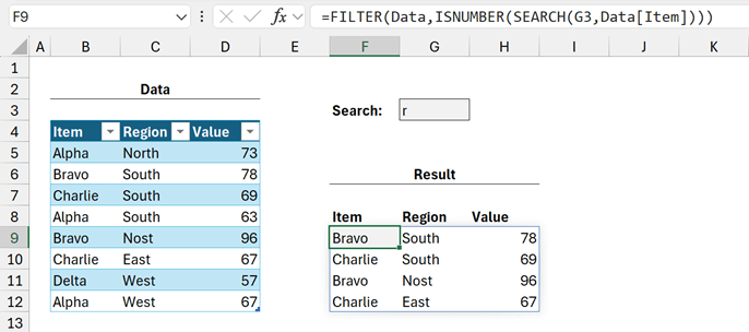
The formula in cell F9 is:

=FILTER(Data,ISNUMBER(SEARCH(G3,Data[Item])))

• SEARCH finds the letter r (value in cell G3) in each Item and returns an array: {#VALUE!;2;4;#VALUE!;2;4;#VALUE;VALUE}
• ISNUMBER checks if each item from SEARCH is a number: {FALSE;TRUE;TRUE;FALSE;TRUE;TRUE;FALSE;FALSE}

Using this inside FILTER, returns only those rows where the Item contains the characters in G3.

Show all if blank search

FILTER is great for creating dynamic reports where users can filter based on different criteria.

However, what if we want an option to show all values? In that scenario, we can use multiple conditions.

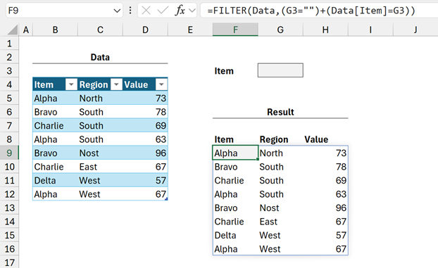
The formula in cell F9 is:

=FILTER(Data,(G3="")+(Data[Item]=G3))

• G3="" checks if the value in G3 (blank) is equal to blank and returns a single value: TRUE
• Data[Item]=G3 checks if each value in the Item column matches with the value in G3 (blank) and returns a value for each row: {FALSE; FALSE; FALSE; FALSE; FALSE; FALSE; FALSE; FALSE}

  Due to an array method known as broadcasting, the single TRUE is applied to each item in the array.

• TRUE + TRUE = 2 (TRUE)
• TRUE + FALSE = 1 (TRUE)
• FALSE + TRUE = 1 (TRUE)
• FALSE + FALSE = 0 (FALSE)

For the include argument in our example:

• Initial calculation: TRUE + {FALSE; FALSE; FALSE; FALSE; FALSE; FALSE; FALSE; FALSE}
• Final Result: {1;1;1;1;1;1;1;1}

Using this approach with FILTER, a blank cell returns all the values from the array.

Filter based on a list

Rather than filtering on single values, we may want to filter on multiple values contained in a list.

For this we can use a MATCH and ISNUMBER combination.

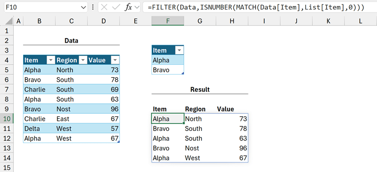
The formula in cell F10 is:

=FILTER(Data,ISNUMBER(MATCH(Data[Item],List[Item],0)))

• MATCH(Data[Item],List[Item],0) looks at each item in the Table and returns the position of the corresponding Item in the List table. If no value is found it returns #N/A. The result for the example is: {1;2;#N/A;1;2;#N/A;#N/A;1}
• ISNUMBER checks if each value calculated by MATCH is a number: {TRUE;TRUE;FALSE;TRUE;TRUE;FALSE;FALSE;TRUE}

Using this inside FILTER allows us to return values based on a list.

If we have the new TEXTSPLIT function, we can also FILTER based on a comma separated list.

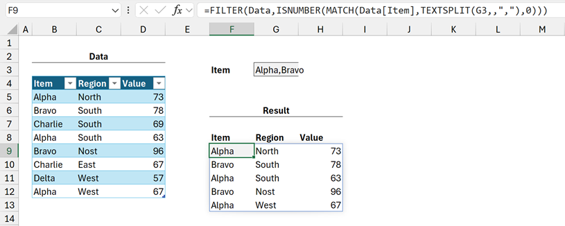
The formula in cell F9 is:

=FILTER(Data,ISNUMBER(MATCH(Data[Item],TEXTSPLIT(G3,,","),0)))

TEXTSPLIT separates each item in the list into a column, which operates as the lookup_array inside the MATCH function.

Filter based on Slicer selection

We can add slicers to a Table to enable quick filtering; the slicer selected items remain visible, while the others are hidden.

SUBTOTAL is a function which ignores hidden rows. Therefore, if we use the COUNTA method of SUBTOTAL, it calculates 1 for each visible cell and 0 for hidden rows.

Unfortunately, SUBTOTAL is an aggregation function, so by itself, it only returns a single value. However, if we wrap SUBTOTAL in a BYROW/LAMBDA combination, it will calculate a value for each row in a range.

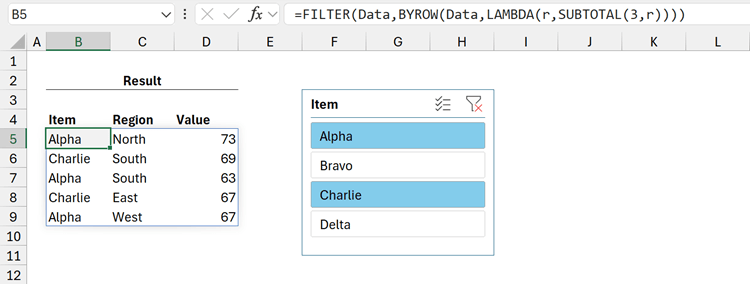
The formula in cell B5 is:

=FILTER(Data,BYROW(Data,LAMBDA(r,SUBTOTAL(3,r))))

• BYROW(Data,LAMBDA(r,SUBTOTAL(3,r))) counts the visible cells in the table: {3;0;3;3;0;3;0;3}

  Using this inside FILTER means we can use slicers to control the FILTER function.

  Notes:

• The COUNTA version of SUBTOTAL returns 3 in this example as there are 3 columns in the array. 3 is a non-zero number, which Excel treats as TRUE.
• As a slicer hides rows, this method works best with the table and formulas are on different tabs.

Conclusion

In this post, we have seen various ways of calculating TRUE or FALSE values to use in the FILTER function. We can combine these techniques to create very powerful filtering functionality in Excel.

Once we realize the include argument is an array of TRUE or FALSE values, and not a list of conditions, it opens up a whole new world of possibilities. Each example in this post serves as a scenario you can use, but also as inspiration for your own ideas.