The underused Table feature in Excel & Google Sheets

Google Sheets finally introduced Tables last month (June 2024), whereas Excel has had them since 2007. There are many overlapping features but some key differences as explained in this article and the table below.

Table benefits

Excel Tables have the following major benefits:

• Formatting is controlled at the table level (like Word or PowerPoint Tables), not the cell-by-cell level
• If a new column to the right is added, the formatting automatically grows, if a new row is added below, everything grows, formats, formulas in that column, data validation etc.
• Formulas linked to the Table have structured references, e.g. =SUM(Events [Sales]) will Sum the Sales column in the Table named “Events”.
• Formulas, PivotTables, charts, data validation lists etc. which have source data in a Table will refer to structured reference e.g. =SUM(Data[Sales] and not cell ranges e.g. =SUM(B4:B9). The key benefit is that the structured reference will grow as new data is added.

Creating Tables in Google Sheets

In Google Sheets, select your data > Format > Convert to Table. Get the sample file here, watch the video here or read more below.

Formatting will make the header row one colour and alternating white/grey for the rows. The Table name will appear on the top left, which is convenient and easy to rename, and click drop downs on the Table name or column headers to access more options. Most column options are as expected such as sort, filter, inserting and deleting but Google’s Tables have a couple of database style features over and above what Excel’s Tables can do such as the ability to set a column type or Group by column.

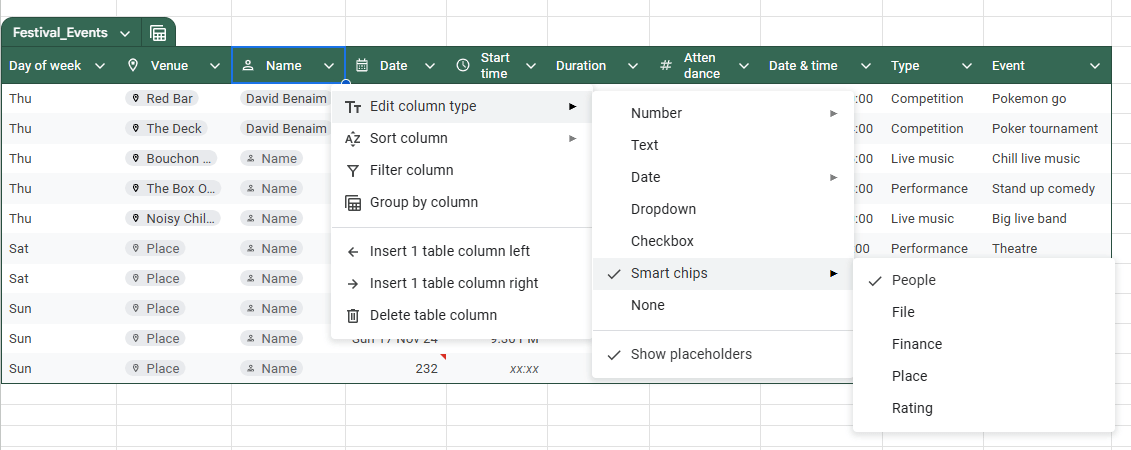
Setting column types in Google’s Tables

Set a column type to date, checkbox, dropdown is similar to Data validation, whilst the text column type is a data format so you can type a phone number without leading zeros being removed, you can also add placeholders for date, time, number. The Smart chip column types take things to the next level:

• People: This contains email addresses/names/photos of people who are in your Gmail contacts
• File: This contains a hyperlink to any file in Google Drive
• Finance: This contains stocks or currency pairs and can extract pricing or other information
• Place: This allows you to search any location in Google Maps
• Rating: This is a 0-5 star rating.

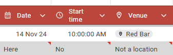
Setting the data type adds an icon on the header but it does not formally become data validation, as you cannot restrict people from typing invalid data. Once they type in invalid data in the column though, they will see a red triangle on the cell. Perhaps a future update will see it officially become data validation.

Group by column in Google Sheets

Many spreadsheet users set up data in a grouped way but this leads to difficulties with filtering, formulas, PivotTables and more. Google now has an option to view Tables grouped by a column, as shown below. There is currently no ability to add subtotals though, which seems like a logical added value feature (explained later in this article for Excel). These views can be saved for easy access later on when clicking the table icon on the top left. Note you can also get to Group by for a non-Table range from the Data menu but clicking that will first make your data into a Table.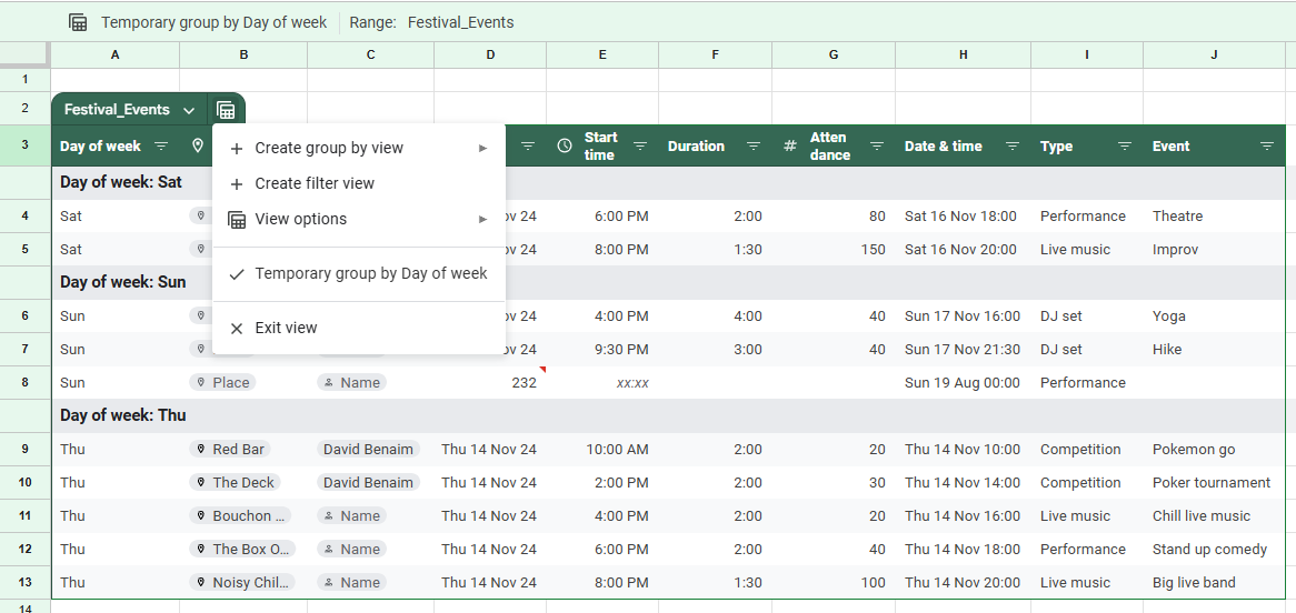

Other Google Sheets Tables features

Resizing, convert to unstructured and format options are available from the dropdown by the Table name, but click Format menu > Alternating colours to adjust the formatting to a more granular level. Clicking Insert menu > Tables gives you dozens of templates of prebuilt tables that users can select, for example product roadmap, inventory trackers, event schedules etc.

Creating Tables in Excel

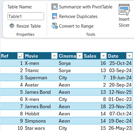
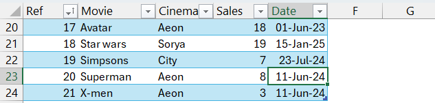
In Excel, select your data > Insert tab > Table, then your data will be reformatted with the header row in dark blue and alternating rows with white and light blue backgrounds as shown. Get the sample file here (click File > Download), read below or watch this video: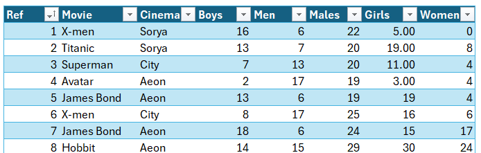

The new Table Design tab will appear on the Ribbon with the ability to change the style or shade different colours for the first column, last column, alternating or banded columns/rows. You can easily toggle the Filters on/off, and a strange option but unticking “Header row” will hide the header row but the column names will still be used in formulas. If you tick “Total Row” (a feature not available in Google Sheets), Excel will add a new row below with different formatting. The bottom left cell will say “Total”, the bottom right cell with show the sum using the SUBTOTAL function, but every other cell has a dropdown where you can choose which aggregation type to use. The total shown will respect any filters, and if you want to grow your table, you can untick the total, grow the table and then put it back.

The left-hand side of the Table Design tab allows you to rename the Table, which is always recommended, you can also insert Slicers (floating filters only available for Tables and PivotTables).

With Excel Tables, you will always see the header row and filter icons, even when the first few rows are not visible, if you click inside the Table, much like the Freeze Panes feature. If you move your cursor to the bottom of a cell in the header row, it will show an arrow, clicking will select the column within the table only.

Structured referencing and formulas for Excel and Google Tables

Many formulas break because cell ranges are hard coded, and rows underneath are not included. These issues mostly go away with Tables in both applications because of structured references whereby the table and column names are referred to in formulas which also makes the formulas easier to understand. Google sheets uses structured references for Table names and Column names using square brackets, whereas Excel additionally has structured references for column headers and the current row which uses @ before the name, and two ]] if there are multiple words in the column headers. Structured references are most useful for column names, for cells in the same row they can be useful, but =[@Sales]-[@[Cost_amount]] can seem like a foreign language aren’t familiar with Tables, which unfortunately is still the vast majority of regular Excel users.

Unstructured	Excel Table	Sheets Table
=SUM(G4:G130)	=SUM(Sales_Table[Sales])	=SUM(Sales_Table[Sales])
=C5-D5	=[@Sales]-[@[Cost_amount]]	=C5-D5
=XLOOKUP(B4, $L$4:$L$8, $M$4:$M$8)	=XLOOKUP([@Employee], People[Name], People[Sales])	=XLOOKUP(B4, People[Name], People[Sales])

Dynamic Array formulas do not work in Excel Tables, whilst many of these formulas would not usually be useful in a Table, some great functions like TEXTSPLIT would be. Google’s Tables have no limitation for dynamic arrays. In Sheets, if the array grows below the Table though, the Table doesn’t expand with it.

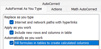
When you create a formula in a column in Google Sheets, it will suggest for you to autofill the column in both an unstructured and a structured table, Excel will do it for you in a Table but will not suggest anything in an unstructured table. Excel allows you to undo calculated column or to stop automatically calculating columns, but if you click the latter its tricky to revert. You must click File > Options > Proofing > Auto correct options > Auto format as you type and ensure all are ticked.

In both applications, relative/absolute references may give unexpected results, if this happens, type in the cell references manually.

Keyboard shortcuts

In Excel, certain shortcuts are slightly different when your active cell is inside a Table, Shift Space which selects the row would select the cells in the row only in the Table (which is very useful), Shift Space again selects every cell in that row. Ctrl A selects the entire Table excluding the header row, Ctrl A for a second time will select the header row too, and a third time will select every cell in the worksheet. Ctrl Space similarly first selects the Table column excluding the header.

In Google Sheets, for Tables or unstructured Table-like range, the behavior is the same, Ctrl/Shift space will also select the column/row until the end of the range including the header, press again to select until the end of the worksheet.

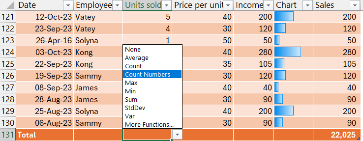
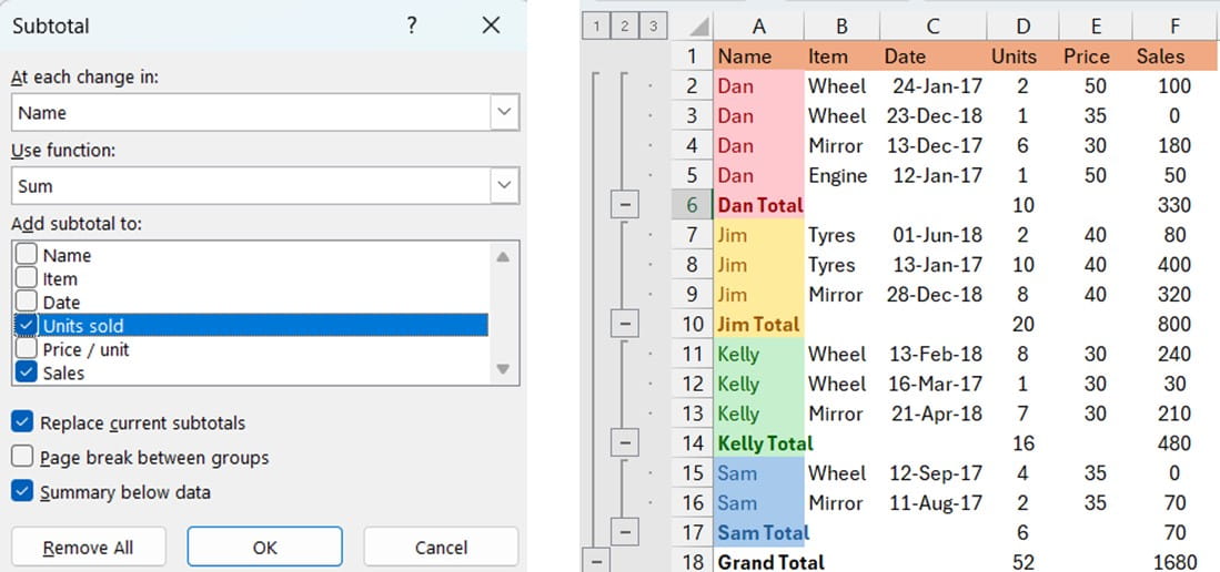
Subtotals in Excel

In Excel, click Data > Subtotal (or Data > Outline > Subtotal on small screens), to automate getting subtotals (possible with 11 functions including sum, average, counts, and statistical ones like variances, standard deviations etc.) using the SUBTOTAL function.

This creates groupings for each category and adds up the specified columns, as opposed to Google Sheets’ version, this changes your data rather than giving you a temporary view, and as such the feature doesn’t work in a Table. More is shown in this video.

Sheets vs Excel Tables comparison of features

Item	Google Tables	Excel Tables	Comments
Auto-grow right & below	Y	Y
Auto-grow when insert col left	Y	N
Conditional formats grow below on expansion	N	Y
Formula autofill in column	Y	Y	In Sheets, its recommended but not automated
Structured refs for entire column & table	Y	Y	The most important of the structured referencing which is easier to understand than those referring to the same row
Structured refs for the same row & headers	N	Y	Good feature in Excel but it makes formulas look like a foreign language
Add new row formulas fill down	Y	Y
Create Pivot from Table	Y	Y
Header row cannot have formulas	Y	Y
Array formulas work as usual	Y	N	Arrays not blocked in Sheets but if the array grows below the table, the table doesn’t expand with it
Rename table	Y	Y	In Sheets, name appears on top left & easy to rename
Assign data type to cols	Y	N	Data types available but not marked as validation and incorrect entries aren't blocked
Placeholders in cells	Y	N	Useful but custom data formats no supported
Smart chip placeholders	Y	N	Places (search on Google Maps) , people (people who emailed), file (from Google Drive) finance (like Stock data types), rating (1-5)
Convert to unstructured data	Y	Y	Excel: Convert to range, Sheets: Convert to unstructured data
Select row/column selects the Table only	Y	Y	Ctrl Space selects without the header in Excel, with header in Sheets
Automatic total row	N	Y	Sheets requires manual total row; Excel can automate it
Move multiple sheets with Tables in them	Y	N
Merged cells blocked	Y	Y
Paste part of a Table will make a Table	Y	N
Header row always visible (like Freeze Panes)	N	Y	Excel freezes only cols
Table name on top left covers 1-2 cells above left side	Y	N	Be aware as you need to plan for it
Group by views	Y	N	Useful, but no subtotals
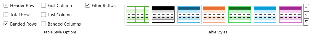
Choosing styles	Y	Y	Easier in Excel (Table tab). Sheets allows header formatting in the Table menu, the rest in Format menu > "Alternating colours"
Filter views	Y	Y	You can access in Sheets without leaving the Table, or in Excel View > Sheet view
Select all omits column headers	N	Y	Sheets has same behaviour as normal for select all