Ticks, crosses and noughts

Introduction

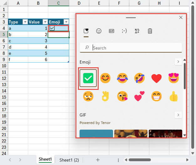
This article was inspired by an excellent tip posted by Jessica S on LinkedIn. It was a very simple, but very useful, tip that either the Windows key+; (semi colon) or Windows key+. (full stop) keyboard shortcut could be used to insert emojis into Excel and other Microsoft Office applications.

Check first…

The original post suggested the use of the technique to enable the entry of a tick as a part of a reconciliation process within Excel as an example of a practical use.

Before launching into the world of emojis, it’s worth remembering that in recent versions of Excel, there is now a way to insert a ‘tickable’ check box into a cell and copy it like any other cell content, making it perhaps the simplest way of dealing with simple tick/no-tick requirements. These in-cell Check Boxes can even be copied automatically as part of a Table column. We have covered this new feature in more detail in a couple of previous articles:

• Excel Tips and Tricks #495 - Excel “Tick”ery!
• Don’t be a check box Charlie

Back to emojis

Returning to our emojis and going beyond the tick/no tick options of a check box, the use of the Windows keyboard shortcut is potentially easier than the use of either the Wingdings font, or the Insert Ribbon tab, Illustrations group, Icons alternative to generate a tick or cross for example. The way in which it works depends on the edition of Excel. In Excel for the Web, the icon is reproduced in colour, whereas in the desktop application it is shown as a black and white outline:

Conditional formatting

After reading the LinkedIn post and experimenting with a few emojis, I started considering whether conditional formatting could provide an even quicker way of entering a tick or similar symbol. Setting a single conditional format for a column could allow a tick – in colour – to be displayed with a single keystroke, rather than the keyboard shortcut plus mouse-click of the emoji method. However, there is the overhead of setting up the conditional format in the first place. It’s worth mentioning that if the conditional format was set up in a Table column, then it should be automatically copied to new rows as they are added to that Table.

Here, we have used a conditional formatting rule to display a green tick for any value greater than 0, with a red cross displayed for any numbers of 0 or below. The setting of ‘Show Icons Only’ has been turned on so that the cell will only display the icon and not the value entered. Note also the ability to choose each of the three Icons, including choosing No Cell Icon, and to change the comparisons, Values and value Type:

Having applied the conditional format to all the required cells, entering a 1, or any other positive number, will cause the cell to display a tick. Entering a zero or negative number will display a cross.

Of course, a formula could also be used to generate the value in the conditional format cell and display the required icon automatically.

Every day is a school day

As well as the potential efficiency of generating the icon, and the ability to use a green tick and red cross rather than just a monochrome icon, I had thought that one of the advantages of generating the icon by using conditional formatting was that the cell would then also have a value that could be used in a formula, in a way that just inserting an emoji could not. It was while investigating this that I learnt something new about illustrations.

In fact, when inserting an illustration in a cell, Excel is able to distinguish different illustrations making it possible to include references to the cells in a formula:

As well as working with references to the cells containing the emojis, it is also possible to include the emoji in the formula directly, but the emoji needs to be enclosed in double quotes:

This would allow an IF() function to be used to choose between emojis based on the value in a cell:

Although Excel illustrations don’t seem capable of being used in a formula in this way (unless anyone knows differently…), it is possible to compare illustrations in cells, even photographs. Here we are comparing two stock image photographs, and we can see that our formula comparison seems, perhaps surprisingly, to work:

Using icons and emojis in column filters and sorts

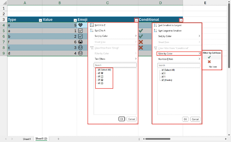
As pointed out in one of the comments to the original LinkedIn post, the emojis work in column filters and sorts, as do Conditional Formatting icons:

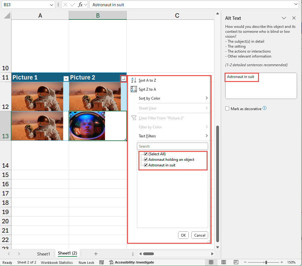
More surprisingly, you can filter and sort by photographic picture as well. In the case of pictures, the Alt Text seems to be used for both operations:

Additional resources

You can explore all aspects of Excel, including many articles on conditional formatting, in the ICAEW archive.