For 2024, I thought I would count down a very subjective “Top 12” of Excel function combinations. And this month’s offering makes it very clear that this is a highly subjective list. If you don’t like this month’s suggestion, that’s fine; life would be boring if we were all in agreement.

Continuing our Top 10 countdown, we are now in the midway through the Top 3. Our runner-up is the highly useful SUMPRODUCT OFFSET.

Let’s consider them individually to begin.

SUMPRODUCT

I must admit this is one of my favourite functions in Excel – so much so our company was named after it (time for a shameless plug)! At first glance,

SUMPRODUCT(vector1, vector2,...)

appears quite humble. Before showing an example, though, let’s look at the syntax carefully:

• A vector for Excel purposes is a collection of cells either one column wide or one row deep. For example, A1:A5 is a column vector, A1:E1 is a row vector, cell A1 is a unit vector and the range A1:E5 is not a vector (it is actually an array, but more on that later). The ranges must be contiguous; and
• This basic functionality uses the comma delimiter (,) to separate the arguments (vectors). Unlike most Excel functions, it is possible to use other delimiters, but this will be revisited shortly below.

Consider the following example:

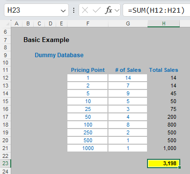
The sales in column H are simply the product of columns F and G, e.g. the formula in cell H12 is simply =F12*G12. Then, to calculate the entire amount cell H23 sums column H. This could all be performed much quicker using the following formula:

=SUMPRODUCT(F12:F21,G12:G21)

i.e. SUMPRODUCT does exactly what it says on the tin: it sums the individual products.

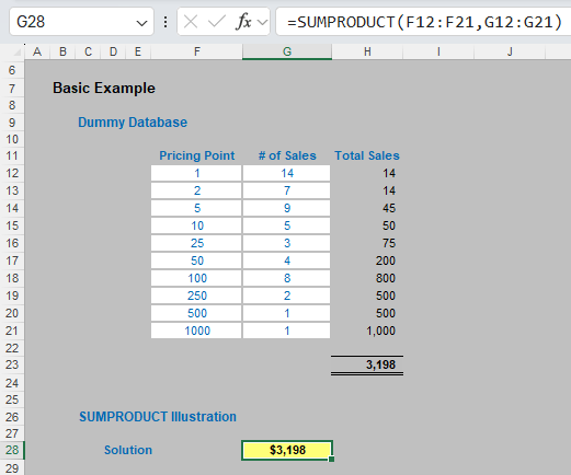
I mentioned the comma delimiter earlier. You can multiply the vectors together instead.

=SUMPRODUCT(F12:F21*G12:G21)

will produce the same result. However, there is an important difference. You can use it to evaluate criteria, e.g.

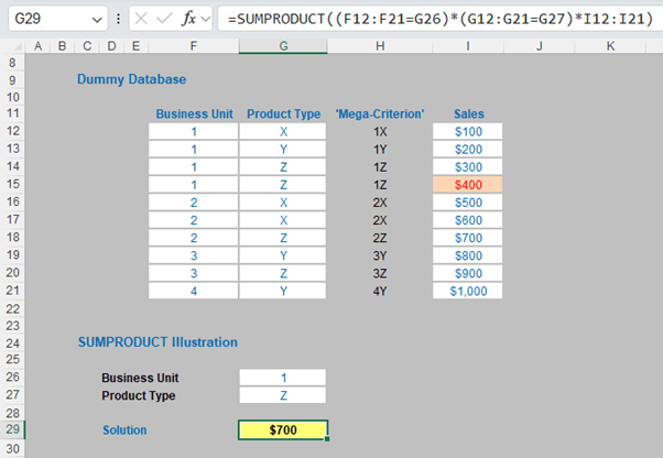
Here, SUMPRODUCT will work with numbers that aren’t really numbers. It comes into its own when dealing with multiple criteria. This is done by considering the properties of TRUE and FALSE in Excel, namely:

TRUE*number = number (e.g. TRUE*7 = 7); and

FALSE*number = 0 (e.g. FALSE*7=0).

Here, (F12:F21=G26) tests to see whether the Business Unit is 1 and (G12:G21=G27) tests to see whether the Product Type is Z. Only if both are TRUE will the Sales figure(s) be added.

OFFSET

I haven’t written about OFFSET for at least one article! As a reminder, the syntax for OFFSET is as follows:

OFFSET(reference, rows, columns, [height], [width]).

The arguments in square brackets (height and width) can be omitted from the formula, but we will require them for this combination.

In its most basic form, OFFSET(reference, x, y) will select a reference x rows down (-x would be x rows up) and y columns to the right (-y would be y columns to the left) of the reference. For example, consider the following grid:

OFFSET(A1,2,3) = 16, viz.

OFFSET(D4,-1,-2) would take us one row up and two columns to the left, returning cell B3. Therefore, OFFSET(D4,-1,-2) = 14, viz.

Furthermore, OFFSET has other practical uses in Excel, taking advantage of the height and width arguments. Consider the OFFSET example from earlier. If we extend the formula to OFFSET(D4,-1,-2,-2,3), it would again take us to cell B3 but then we would select a range based on the height and width parameters. The height would be two rows going up the sheet, with row 14 as the base (i.e. rows 13 and 14), and the width would be three columns going from left to right, with column B as the base (i.e. columns B, C and D).

Hence OFFSET(D4,-1,-2,-2,3) would select the range B2:D3, viz.

Note that OFFSET(D4,-1,-2,-2,3) equals #VALUE! in legacy Excel as it cannot display a matrix in one cell, but it does recognise it, as evidenced in Excel 365 where it will spill as a dynamic array.  Dynamic arrays are something of a prerequisite for this book, but if you do find yourself using OFFSET in earlier versions of Excel, help is at hand. If it does not display, after typing in OFFSET(D4,-1,-2,-2,3) we press CTRL + SHIFT + ENTER, we turn the formula into an array formula: {OFFSET(D4,-1,-2,-2,3)} (do not type the braces in, they will appear automatically as part of the Excel syntax). This gives a value of 8, which is the value in the top left-hand corner of the matrix, but even the earlier versions of Excel are storing more than that. This can be seen as follows:

• SUM(OFFSET(D4,-1,-2,-2,3)) = 72 (i.e. SUM(B2:D3))
• AVERAGE(OFFSET(D4,-1,-2,-2,3)) = 12 (i.e. AVERAGE(B2:D3)).

SUMPRODUCT OFFSET

To illustrate the usefulness of SUMPRODUCT OFFSET in financial modelling, let’s consider the following example:

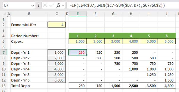
The above is known as a depreciation grid.  Cells C7:C12 transpose the values in cells E5:J5 using the OFFSET function (e.g. the formula in cell C7 is =OFFSET($D$5,,$B7), given the contents of cells B7:B12 are simply numbers made to look like text using number formatting). The formula in the grid (e.g. cell E7) is: 

=IF(E$4<$B7,,MIN($C7-SUM($D7:D7),$C7/$C$2))

This calculates the depreciation amount assuming the period is a period where depreciation should be calculated. The grid is great for explaining how depreciation works. Users understand the logic without looking at the formula – which is probably just as well given what lurks beneath. There is a major disadvantage with this method though. A few years back, I had to construct several hundred depreciation calculations where users required monthly calculations for a 20-year period. That means each grid had 240 columns and 240 rows, i.e. 57,600 calculations per grid. Yuck!

There is a shorter method, using a SUM(OFFSET) method – which is halfway to our SUMPRODUCT OFFSET combination. Look at the following alternative calculation:

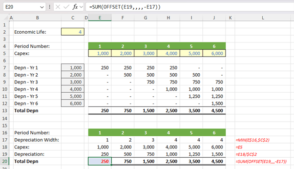
It may not look intuitive to begin with but allow me to talk you through it.

• Row 17 takes the minimum of the period counter and the economic life. This formula is used to determine how many periods need to be considered. The maximum number of periods is 4 here, so that no year’s capital expenditure may be over-depreciated.
• Row 18 simply restates the capital expenditure from row 5.
• Row 19 is another simple formula: it simply takes the capital expenditure figure and divides it by the economic life (I have simplified the formula in this example, in a real model we would need to ensure that the economic life is a positive integer).
• Row 20 simply uses the SUM(OFFSET) approach to add up amounts. The formula in cell E20,

=SUM(OFFSET(E19,,,,-E17))

starts with the Depreciation in cell E19 and does not move any rows or columns. Given the height parameter is unspecified it is assumed to be 1 (i.e. just row 19) but the width parameter is -1. A width of 1 or -1 simply means the column you are in so for the first period, the amount is simply =SUM(250) which equals 250.

For F20, the OFFSET function starts in cell F19, does not move anywhere, has a height of 1 and a width of -2, which is column F and the column to the immediate left (E). The formula evaluates to =SUM(500+250) which equals 750.

Moving on, cell I20 (Period 5) takes the sum of the value in cell I19 and the three cells to the left. This formula evaluates to =SUM(1250+ 1000+750+500) which equals 3,500.

This method is shorter, but perhaps not quite so transparent. 

Let’s now extend the SUM OFFSET idea for depreciation. This works fine if the rate remains constant, but what happens if it can change each period (i.e. you are using just about any other depreciation method)?

This is the “universal” formula but is conceptually even more complex than SUM(OFFSET). This uses SUMPRODUCT(OFFSET,OFFSET). Consider the following example:

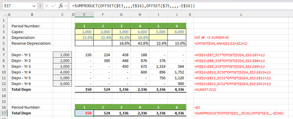
In this example, I have made the depreciation methodology the “Liam Random Method” where I have put arbitrary percentages in cells E4:I4, with J4 the balancing figure. Ignoring row 5 for a moment, the depreciation grid in rows 7:13 calculates the depreciation on a period-by-period basis using the formula: 

=IF(E$2<$B7,,$C7*OFFSET($D$4,,E$2-$B7+1))

in cell E7 for instance. This formula may look terrible, but the first argument determines whether depreciation should be calculated as in my previous example and the OFFSET calculation simply ensures the right percentage is used in each period as the percentages ‘move’ depending upon which row you are in. You will admit though it is not the world’s simplest calculation even though it is still fairly easy to understand if the calculation were simply printed out.

We can get a lot smarter though.

• Consider the Total Depreciation in cell E13. This is simply 1,000 x 15%, which is =E3*E4 or =SUMPRODUCT(E3,J5) (even if this does look like over the top).
• Now examine the Total Depreciation in cell F13. This is (1,000 x 22.4%) + (2,000 x 15%) or =SUMPRODUCT(E3:F3,I5:J5).
• I shall keep going. Look at the Total Depreciation in cell G13. This is (1,000 x 43.8%) + (2,000 x 22.4%) + (3,000 x 15%) or =SUMPRODUCT(E3:G3,H5:J5).

Do you see where I am going? By reversing the depreciation rates in row 4 using the formula

=OFFSET($D4,,MAX($2:$2)-E$2+1)

in cell E5 for instance, I have a row vector that I can cross-multiply with the Capex in row 3 using the SUMPRODUCT function. The final argument in the formula above merely moves the reference MAX($2:$2)-E$2+1 columns to the right. This effectively moves Period 1 to Period 6, Period 2 to Period 5 and so on.

I may get more and more product formulae depending upon the number of periods, but the SUMPRODUCT formula remains fairly simple, once someone has explained it. The formula in cell E17 is actually not that bad:

=SUMPRODUCT(OFFSET($E3,,,,E$16),OFFSET($J5,,,,-E$16))

It may look horrible to start off with, but it’s not that bad when considered systematically. The two OFFSET functions simply keep expanding the two row vectors, the first further right and the second further left. It won’t actually be long before this formula is simpler than its long hand equivalent which will not even be a consistent formula period to period.

Word to the Wise

SUMPRODUCT OFFSET is frequently used in spreadsheets to aggregate depreciation and working capital, where amounts may vary period to period. Whilst it seems unnecessarily complex when you first encounter it, this combination can save a lot of file size and memory when there are many similar depreciation or working capital calculations.

The top 3 continues next month.