For 2024, I thought I would count down a very subjective “Top 12” of Excel function combinations.  And this month’s offering makes it very clear that this is a highly subjective list.  If you don’t like this month’s suggestion, that’s fine; life would be boring if we were all in agreement.

Continuing our Top 10 countdown, we are now firmly entrenched in the Top 5.  The 4th of 12 is another dynamic array combination: SORT UNIQUE – so again, sorry, it’s only in Excel 365, but maybe this is a good reason to switch if you haven’t already.

Let’s look at the functions individually first of all.

SORT

The SORT function sorts the contents of a range or array:

=SORT(array, [sort_index], [sort_order], [by_column]).

It has four arguments:

• array: this is required and represents the range that is required to be sorted
• sort_index: this is optional and refers to the position of the row or the column in the selected array (e.g. second row, third column).  99 times out of 98 you will be defining the column, but to select a row you will need to use this argument in conjunction with the fourth argument, by_column.  And be careful, it’s a little counter-intuitive!  The default value is one [1]
• sort_order: this is also optional.  The choices for sort_order are 1 for ascending order (default) or -1 for descending.  It should be noted that you might not want to hold your breath waiting for ‘Sort by Color’ (sic), ‘Sort by Formula’ or ‘Sort by Custom List’ using this function
• by_column: this final argument is also optional.  Most people want to sort rows of data, so they will want the value to be FALSE (which is the default value if not specified).  Should you be booking your mental health check, you may wish to use TRUE to sort by column in certain instances.

To show you how simple it is, consider the following data:

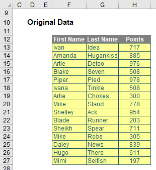
Sorting the ‘Points’ column in order is as easy as this:

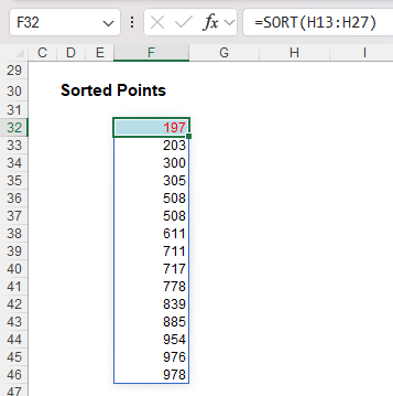
All you do is type =SORT(H13:H27) into cell F32.  That’s it!  Note that the duplicates are repeated; there is no cull.  If you want it in descending order, simply specify the requirement in the formula:

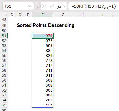
This formula is only slightly more sophisticated, in that the sort_order (third argument) needs to be specified as -1 to switch the sort to descending order:

=SORT(H13:H27,,-1).

You probably won’t want the points displayed on their own:

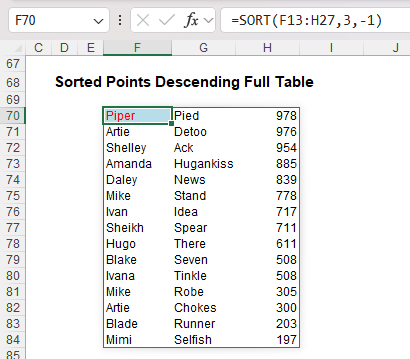
Now all of these arguments start to make more sense.  SORT(F13:H27,3,-1) produces the whole array (array is F13:H27), sorts it on the third (sort_index is 3) column in descending (sort_order is -1) order.  Blake and Ivana tie on 508 points, but Blake appears first as he was first in the original (source) table.

So far, I have only performed the one SORT.  You can have more than one though:

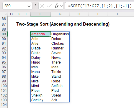
Here, I have created a second (two-level) SORT.  Here, you need to create what is known as an array constant for the second and third arguments (you just type the braces in – don’t use CTRL + SHIFT + ENTER):

=SORT(F13:G27,{1;2},{1;-1}).

This will sort on column 1 (‘First Name’) first, then sort on column 2 (‘Last Name’) next.  This will be in ascending order (1) for the first column and descending order (-1) for the latter.  It’s not as straightforward a formula entry as most Excel modellers are used to, but it’s relatively painless once you have committed it to erm, um, what do you call it, memory.

UNIQUE

Weirdly, UNIQUE does two things (!).  It details distinct items (i.e. provides each value that occurs with no repetition) and also it can return values which occur once and only once in a referred range.  I understand that Excel users may welcome the former use with open arms and that database developers may be very interested in the latter.

The UNIQUE function has the following syntax:

=UNIQUE(array, [by_column], [occurs_once]).

It has three arguments:

• array: this is required and represents the range or array from which to return unique values
• by_column: this argument is optional.  This is a logical value (TRUE / FALSE) indicating how to compare.  If you wish to compare by row, the argument should be FALSE or omitted (since this is the default).  To compare by column, you will need to select TRUE
• occurs_once: this argument is also optional.  This requires a logical value too:
• TRUE: only return unique values that occur once
• FALSE: include all distinct values (default if omitted).

It’s probably clearer with some examples.  Let’s give it a go.  As always, I need source data:

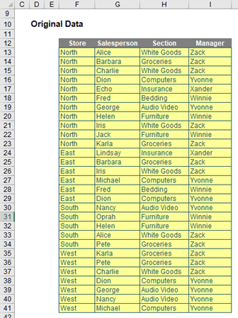
Time for the most basic illustration:

In cell L13, I have simply typed

=UNIQUE(F13:F41).

No optional arguments; everything in default.  If I have made an error, it’s going to be my default.  This has simply listed each store that appears; if “North” and “North ” (extra space) were there, then both would appear.  UNIQUE is not case sensitive though and each entry would appear as it first occurs reading down the range F13:F41.  The other columns contain similar formulae and UNIQUE looks like it takes seconds to learn.

It’s just as simple if you want to see unique records for two (or more) columns, viz.

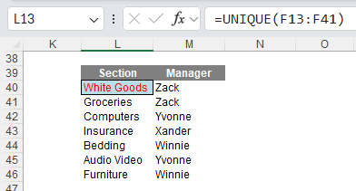
You can see UNIQUE is sort of crying out for SORT, but we’ll get to that shortly.

As mentioned earlier, it’s not the only way of using UNIQUE (no, having a unique use would be just what “they” were expecting, whoever “they” are…).  You can use it to determine values that only occur once:

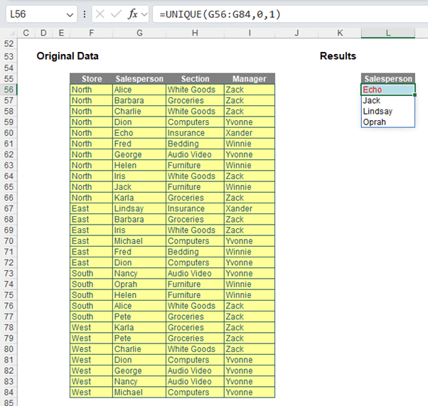
Here, the formula in cell L56,

=UNIQUE(G56:G84,0,1)

uses the non-default value of 1 for the optional occurs_once (third) argument.  This means it identifies the salespeople who only occur once in cells G56:G84.

SORT UNIQUE

There isn’t really much more to add regarding SORT UNIQUE: it merely sorts unique lists.  Rather than show another sorted list, I thought I would end by adding further complexity instead.  The real power starts coming when you start playing with Excel’s existing functions and features, together with these new functions.  Take this comprehensive example:

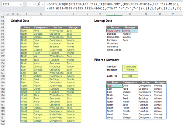
Let me step you through some of this.  The formulae in cells L94 and M94 use UNIQUE in a similar manner to previous example shown, to generate the list of distinct values in the ‘Section’ and ‘Manager’ fields.  However, did you notice they have been sorted?  That’s because I used the formula

=SORT(UNIQUE(H94:H122))

in cell L94, for example.  But then I continued.  The ‘AND / OR’ dropdown is a bit of an anti-climax after that, but the final formula that generates the final table, namely

=SORT(UNIQUE(FILTER(F93:I122,IF(M108="OR",(H93:H122=M105)+(I93:I122=M106),

(H93:H122=M105)*(I93:I122=M106)),{"N/A","-","-","-"})),{1;2;3;4},{1;1;1;1})

is rather fun.  I am not going to go through it though as this article is intended to summarise SORT and UNIQUE.  See if you can work your way through it for yourself.

Word to the Wise

Don’t worry; that is the end of our dynamic arrays, LAMBDAs and Excel 365 features.  Our final examples starting next month will work in all versions of Excel.

The top 3 gets underway next month.