Top 12 Excel Combinations: 6. MAP LAMBDA

For 2024, I thought I would count down a very subjective “Top 12” of Excel function combinations. And this month’s offering makes it very clear that this is a highly subjective list. If you don’t like this month’s suggestion, that’s fine; life would be boring if we were all in agreement.

Continuing our Top 10 countdown, we’re over halfway. The 6^th of 12 is a relatively new combination only available in Excel 365.

As always, I need to introduce the two functions individually, but this time, I shall be doing it in reverse order.

LAMBDA

Only available in Excel 365, LAMBDA “completes” Excel and allows you to define your own custom functions using Excel’s formula language. Moreover, one function can call another (including itself!), so there is no limit to the power you can deploy with a single function call. Additionally, you can use other functions (which we’ll get to shortly) to apply these functions in more versatile ways. This will be essential to building up our financial model later in the book.

One of the more challenging parts of working with formulae in Excel is that you often get fairly complex formulae that are re-used numerous times through the sheet (often by just copying / pasting). This can make it hard for others to read and understand what’s going on, put you more at risk of errors, and make it harder to find and fix the errors. With LAMBDA, you have reusability and composability. You can create libraries for any pieces of logic you plan to use multiple times, which offers convenience and reduces the risk of errors.

Some people are put off by LAMBDA and “lambda”. A lambda function (sometimes referred to as a “Small Anonymous Function”) is IT parlance for a self-contained block of functionality that is transferrable / portable throughout your code.

Think of Excel formulae as your “code”. You can create a user-defined function (a lambda function) using the Excel function LAMBDA to define it. Clear as mud, yes?

So how does it work?

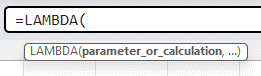
The syntax of LAMBDA is perhaps not the most informative:

That’s, er, great. Its syntax suffers because it is so flexible. Perhaps a run-through might be best. There are three key pieces of LAMBDA to understand:

1. LAMBDA function components
2. Naming a lambda
3. Calling a lambda function

Let’s go through these steps.

1. LAMBDA function components

I will begin with a simple example. Consider the following formula:

=LAMBDA(x, x+1)

where we have x as the argument, which you may pass in when calling the LAMBDA, and x+1 is the logic / operation to be performed. For example, if you were to call this lambda function and define x as equal to five [5], then Excel would calculate

5 + 1 = 6

Except it wouldn’t. If you tried this, you would get #CALC!

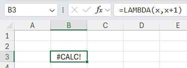
Oops. That’s because it’s not quite as simple as that. There are two [2] ways to fix this. The first is to name your LAMBDA.

2. Naming a LAMBDA

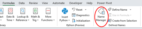
To give your LAMBDA a name so it can be re-used, you must use the Name Manager (CTRL + F3 / go to the Ribbon and then go to Formulas -> Name Manager):

Once you open the ‘Name Manager’ you will see the following dialogue:

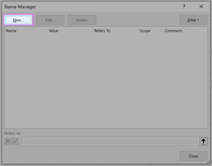
You then click on ‘New’ and fill out the related fields, viz.

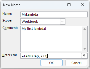
It’s no harder than clicking ‘OK’ at this point.

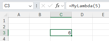
3. Calling LAMBDA

Now that you have done this, your first new lambda function may be called in just the same way as every other Excel function is cited, eg,

=MyLambda(5)

which would equal six [6] and not #CALC! as before.

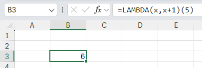
You DON’T have to do it this way though if you don’t want to. You may call a lambda without naming it, and this is the second way to fix the #VALUE! error we had earlier. If we hadn’t named this marvellous calculation, and simply authored it in the grid as we had first attempted, we could call it by simply typing:

=LAMBDA(x, x+1)(5)

As you become more experienced and your expertise grows, you will realise that some transformations may be cumbersome using the functions you already know from “legacy Excel”. For instance, you might find the following awkward:

• combining arrays;
• shaping arrays; and
• resizing arrays.

This where a set of “lambda helper functions” come into play. These allow you to write lambdas more easily. One such helper function is MAP…

MAP

The MAP function returns an array formed by mapping each value in the array(s) to a new value and applying a LAMBDA to create a new value accordingly. It has the following syntax:

MAP(array1, lambda or array2, [lambda or array3, …])

where:

• array1: this is a required argument and represents the (first) array to be mapped.
• array2 and subsequent arrays: these are optional arguments and represent additional arrays to be mapped.
• lambda: this is a required argument which represents a LAMBDA which must be the final argument and must have a parameter for each array passed or another array to be mapped.

In short, MAP transforms values. Consider the following table of data called Temps:

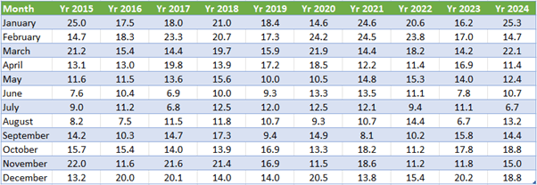
Now this article is not about FILTER, BYROW or AVERAGE, so please just accept that the formula

=FILTER(Temps, BYROW(Temps, LAMBDA(year, AVERAGE(year) > 15)))

will return the following array:

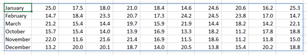
Imagine you wished to convert – transform – this data to Fahrenheit, so our US colleagues may better understand. All I need to do is wrap the above formula in a MAP function:

=MAP(FILTER(Temps, BYROW(Temps, LAMBDA(year, AVERAGE(year) > 15))),
LAMBDA(temperature, IF(ISNUMBER(temperature),
CONVERT(temperature, "C", "F"), temperature)))

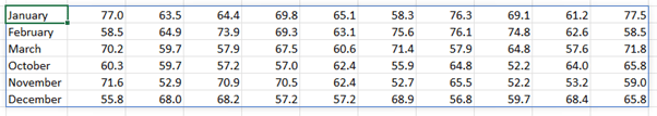
CONVERT(temperature, "C", "F") simply converts the variable temperature from degrees Celsius to degrees Fahrenheit. This is wrapped in an IF(ISNUMBER()) check to ensure that we don’t try to convert text values (as this would cause an error): the IF statement leaves the value of temperature “as is” in this instance, and LAMBDA just wraps around all of this in order to declare the variable temperature, so that MAP may do its work.

It’s true you could generate this result in stages, but the whole idea of these LAMBDA helper functions is to be able to create dynamic arrays in one fell swoop. Therefore, MAP should always be used with LAMBDA – but I want to focus on why this is so useful with a simpler illustration.

MAP LAMBDA

Consider the following example where I have generated a list of numbers from one [1] to five [5] through the use of the SEQUENCE dynamic array function (column C) and hardcoded the first five [5] letters of the alphabet next to this in column D:

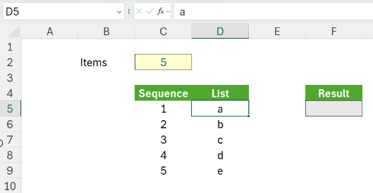
I want to make use of the OFFSET function (mentioned in my last article) in cell F5 to return a list of our letters (I appreciate that there are easier ways to do this without the use of the OFFSET function, but those ways wouldn’t work for our depreciation calculation!). Simply using the formula:

=OFFSET(D4,C5#,)

does not give us the desired result.

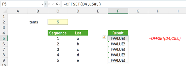
OFFSET and dynamic arrays simply do not work like that: we will have to use a MAP(LAMBDA) function. The formula we must use is:

=MAP(C5#,LAMBDA(x,OFFSET(D4,x,)))

This will perform the LAMBDA function for each value in the array C5#, first offsetting cell D4 by one [1] row and returning “a”, then by two [2] rows and returning “b”, and so on for each value in C5#.

This trick has to be employed all the time when using dynamic array formulae – hence MAP LAMBDA’s popularity!

Word to the Wise

If you don’t have dynamic arrays or Excel 365, it is still a good idea to consign this combination to the memory banks. Excel is evolving and dynamic arrays are likely to become more and more pertinent. Knowing tricks such as MAP LAMBDA will make mastering forecasting and modelling using dynamic arrays just that little bit easier.

Top 5 starts next month.