For 2024, I thought I would count down a very subjective "Top 12" of Excel function combinations. And this month’s offering makes it very clear that this is a highly subjective list. If you don’t like this month’s suggestion, that’s fine; life would be boring if we were all in agreement.

Continuing our Top 10 countdown, the 7^th of 12, is a combination which is regularly used – and hence makes the list – arguably, shouldn’t be. Allow me to explain.

As always, allow me to begin by introducing the two functions in question. (Here is the example spreadsheet).

OFFSET

The older I get, the more invaluable OFFSET becomes. The syntax for OFFSET is as follows:

OFFSET(reference, rows, columns, [height], [width]).

The arguments in square brackets (height and width) can be omitted from the formula (for the purposes of this article, these do not need to be discussed).

In its most basic form, OFFSET(reference, x, y) will select a reference x rows down (-x would be x rows up) and y columns to the right (-y would be y columns to the left) of the reference. For example, consider the following grid:

OFFSET(A1,2,3) would take us two rows down and three columns across to cell D3. Therefore, OFFSET(A1,2,3) = 16, viz.

OFFSET(D4,-1,-2) would take us one row up and two columns to the left, returning cell B3. Therefore, OFFSET(D4,-1,-2) = 14, viz.

We can use these mechanics to construct a very simple scenario table:

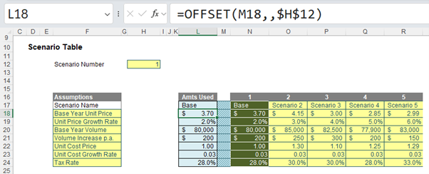
Essentially, the assumptions used in this illustration are linked from cells L18:L24 (in light blue). These values are drawn from the scenario table to the right of the highlighted yellow range (eg, cells N18:N24 constitute Scenario 1, cells O18:O24 constitute Scenario 2).

The Scenario Selector is located in cell H12. Using OFFSET scenarios may be selected at will. For example, the formula in cell L18 is simply OFFSET(M18,,$H$12), that is, start at cell M18 and displace zero rows down and the value in H12 columns across. In the image above, the formula locates the cell one column to the right, which is Scenario 1.

The advantage of OFFSET over other functions such as INDEX, CHOOSE and LOOKUP is that the range of data can be added to. Whilst the other functions require a specified range, with OFFSET we can keep adding scenarios without changing the formula / making the model inefficient.

There are a couple of problems with OFFSET.

The first issue is that the values returned by an OFFSET function confuse Excel. Only the original reference is recognised as a precedent reference to the formula by Excel’s auditing tools.

The result returned is most likely to come from another cell which will not be highlighted by this technique. If you think about it, this actually makes sense as potentially all of the cells on a worksheet are potential precedents.

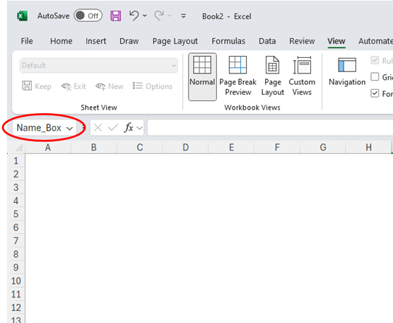
To take account of this, I suggest you give the reference a range name. To name a cell simply, click on the cell and then type the desired name in the ‘Name box’ in Excel:

This range name should start with BC_. This prefix stands for “Base Cell” and makes it easier to sort / locate range names later. When users or model auditors alike inspect a formula with a Reference starting with BC_ for Base Cell (eg, BC_Example_Reference), this can alert them to the fact that the model may be using cells in the region of this Reference that do not appear to have any dependents.

The other issue is that OFFSET is what is known as a volatile function. A volatile function is one that causes recalculation of the formula in the cell where it resides every time Excel recalculates. This can really slow down your model if there are too many OFFSET functions, for example – so use with caution.

MATCH

MATCH(lookup_value, lookup_vector, [match_type]) returns the relative position of an item in an array that (approximately) matches a specified value. It is not case sensitive.

The third argument, match_type, does not have to be entered, but for many situations, I strongly recommend that it is specified. It allows one of three values:

• match_type 1 [default if omitted]: finds the largest value less than or equal to the lookup_value – but the lookup_vector must be in strict ascending order, limiting flexibility;
• match_type 0: probably the most useful setting, MATCH will find the position of the first value that matches lookup_value exactly. The lookup_array can have data in any order and even allows duplicates; and
• match type -1: finds the smallest value greater than or equal to the lookup_value – but the lookup_array must be in strict descending order, again limiting flexibility.

When using MATCH, if there is no (approximate) match, #N/A is returned (this may also occur if data is not correctly sorted depending upon match_type).

MATCH is fairly straightforward to use:

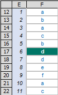
In the figure above, MATCH("d",F12:F22,0) gives a value of 6, being the relative position of the first ‘d’ in the range. Note that having match_type zero [0] here is important. The data contains duplicates and is not sorted alphanumerically. Consequently, using match_type 1 and -1 would give the wrong answer: 7 and #N/A respectively.

OFFSET and MATCH

The power of combining OFFSET with MATCH can be seen with the following example, where I return to the scenario illustration presented earlier:

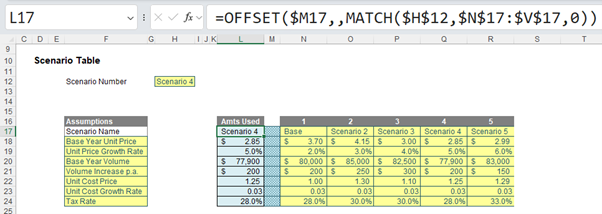
Here, do you see that instead of having a selection number, cell H12 has the Scenario Name (row 17). Therefore, the formula

MATCH($H$12,$N$17:$V$17,0)

is required to identify which position the Scenario Name is in the list in order to know how far to OFFSET the reference, here cell M17 (which is being displaced four columns to the right as a consequence of the result of the MATCH formula.

Indeed, the idea may be extended to a so-called “two-way lookup”, eg,

Here, the formula

=OFFSET(F12,MATCH(G29,F13:F24,0),MATCH(G30,G12:I12,0))

determines both the number of rows down (MATCH(G29,F13:F24,0)) and the number of columns to the right (MATCH(G30,G12:I12,0)) the result should be taken from the reference cell, F12.

Word to the Wise

So why am I arguing OFFSET MATCH shouldn’t be used? Aside from the volatility concerns mentioned earlier, OFFSET is perhaps the wrong function for this scenario (pun intended). OFFSET is a highly versatile function that allows you to extend ranges, such as adding more financial data or invent new months in the final example. The problem is, MATCH doesn’t. It requires a range specified, which rather stunts OFFSET’s growth.

There are more appropriate functions to use in this instance. There is little real benefit using OFFSET with MATCH, unless the vector range in MATCH is a dynamic array. However, that’s not the point of this article; here, I am only highlighting what modellers use, regardless of its merits.

So what might be a better function combination to use? I have a feeling that it might be mentioned in a later article in this series. Keep holding on to those tenterhooks…

The list continues next month.