Top 12 Excel Combinations: 8. INDEX SEQUENCE

For 2024, I thought I would count down a very subjective “Top 12” of Excel function combinations. And this month’s offering makes it very clear that this is a highly subjective list.  If you don’t like this month’s suggestion, that’s fine; life would be boring if we were all in agreement.

Continuing our Top 10 countdown, the 8th of 12, is a combination which may only be used online and with Excel 365. Again, it may often be swapped for simpler calculations, but is useful nonetheless, in certain instances.

Let’s look at the two functions individually first of all.

INDEX

Essentially,

INDEX(array, row_number, [column_number])

returns a value or the reference to a value from within a table or range (list).  For example, INDEX({7,8,9,10,11,12},3) returns the third item in the list {7, 8, 9, 10, 11, 12}, i.e. 9.  This could have been a range: INDEX(A1:A10,5) gives the value in cell A5, etc.

INDEX can work in two dimensions as well (hence the column_number reference).  Consider the following example:

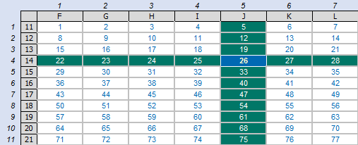
INDEX(F11:L21,4,5) returns the value in the fourth row, fifth column of the table array F11:L21 (clearly 26 in the above illustration).  Interestingly,

=INDEX(J11:J21,0)

will actually return the spilled values contained within cells J11:J21 too (in this instance, down a column as the range is a column vector).

SEQUENCE

This function allows you to generate a list of sequential numbers in an array, such as 1, 2, 3, 4.  It doesn’t sound particularly exciting, but again, it really ramps up when combined with other functions and features, such as INDEX. Its syntax is given by:

=SEQUENCE(rows, [columns], [start], [step]).

It has four arguments:

• rows: this argument is required and specifies how many rows the results should spill over
• columns: this argument is optional and specifies how many columns (surprise, surprise) the results should spill over.  If omitted, the default value is 1
• start: this argument is also optional. This specifies what number the SEQUENCE function should start from.  If omitted, the default value is 1
• step: this final argument is also optional. This specifies the amount each number in the SEQUENCE should increase by (the “step”).  It may be positive, negative or zero.  If omitted, the default value is 937,444.  Wait, I’m kidding; it’s 1. They’re very unimaginative down in Redmond.

Therefore, SEQUENCE can be as simple as SEQUENCE(x), which will generate a list of numbers in a column: 1, 2, 3, …, x.  Therefore, be mindful not to create a formula where x may be volatile and generate alternative values each time it is calculated, e.g. =SEQUENCE(RANDBETWEEN(10,99)) as this will generate the #SPILL! error as the range is volatile in size.

A vanilla example is rather bland:

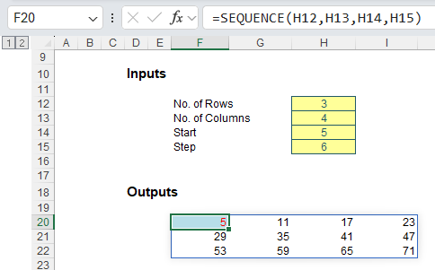
Do you see how SEQUENCE propagates across the row first and then down to the next row, just like reading a book?  I wonder how that might work in alternative languages of Excel where users read right to left (it has to be the same or there would be chaos when workbooks were shared!).

As I mentioned above, SEQUENCE is arguably more powerful when included in a more complex formula.  For example:

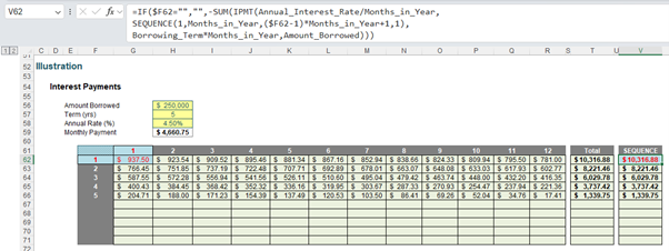
In this instance, I have created a grid using the Excel IPMT function to determine the amount of interest to be paid in each monthly instalment.  Cells G62:R71 calculate each monthly amount and column T sums these amounts to calculate the annual interest payment, a figure which is non-trivial to compute.  The whole table may be replaced by the formula in cell V62:

=IF($F62="","",-SUM(IPMT(Annual_Interest_Rate/Months_in_Year,
SEQUENCE(1,Months_in_Year,($F62-1)*Months_in_Year+1,1),
Borrowing_Term*Months_in_Year,Amount_Borrowed))).

INDEX and SEQUENCE

To be honest, I have never combined these functions (other than in the examples presented), but that is not the point of this series.  I know many users who have – and that is the key point here.

I mentioned earlier that =INDEX(J11:J21,0) will spill.  Hence, INDEX is unlike other functions such as SUM, OFFSET, MIN and MAX which “coerce”, i.e. a range will aggregate to one value displayed in one cell.  Therefore, INDEX can be used to pick different values for different cells using a nested function such as SEQUENCE.

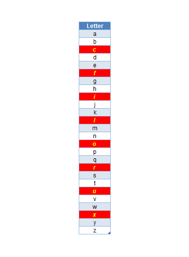
For example, in our attached Excel file, consider the following Excel (CTRL + T) Table called Alphabet:

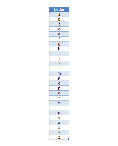
Imagine I wanted to create a list of every third item in this list (highlighted in red), viz.

I could create an input cell, named N_Value which I give a value of three [3] and then write the following formula:

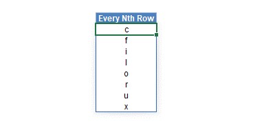
=INDEX(Alphabet[Letter],SEQUENCE(INT(ROWS(Alphabet[Letter])/N_Value))*N_Value)

This would produce the following result:

So how does this work?

ROWS(Alphabet[Letter])

This internal expression calculates the number of rows in the Letter field of the Alphabet Table (26).

INT(ROWS(Alphabet[Letter])/N_Value)

This takes the integer value of 26 divided by 3, which is eight [8].

SEQUENCE(INT(ROWS(Alphabet[Letter])/N_Value))

This generates the sequence of integers from one [1] to eight [8]:

{1, 2, 3, 4, 5, 6, 7, 8}

The expression

SEQUENCE(INT(ROWS(Alphabet[Letter])/N_Value))*N_Value

simply multiplies this sequence by N_Value, which is three [3]:

{3, 6, 9, 12, 15, 18, 21, 24}

Thus,

=INDEX(Alphabet[Letter],SEQUENCE(INT(ROWS(Alphabet[Letter])/N_Value))*N_Value)

takes the third, sixth, ninth, etc. value in the Letter field.

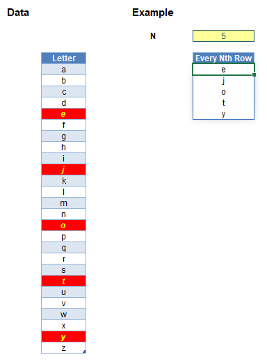
It works similarly for other values of N_Value, such as every fifth item:

Rather than pick every Nth item, you can also get INDEX SEQUENCE to repeat references or act like a FILTER function.  Let me explain with another example (from the same Excel file).

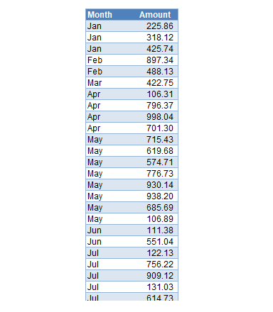
Imagine I have another Excel (CTRL + F3) Table called Data:

Imagine I selected one of the months, say “Jan”, using an input cell, viz.

Here, I have named the input cell Month_Selected, and the cell below (named Occurrences) counts the number of times “Jan” appears in the Month field of the Data Table:

=COUNTIF(Data[Month],Month_Selected)

I want to create the following Table:

This may be achieved very simply using the dynamic array function FILTER as follows:

=FILTER(Data,Data[Month]=Month_Selected)

Here, the Table Data is formulaically filtered such that the value in the Month filed is “Jan”.  Easy.

Of course, I want to find a more awkward way of doing this using INDEX SEQUENCE expression!

For the Month, I use the following expression:

=INDEX(Month_Selected,SEQUENCE(Occurrences,,1,0))

Here, SEQUENCE(Occurrences,,1,0) generates three [3] values of one [1]:

{1, 1, 1}

Therefore, the “range” Month_Selected simply takes the first cell and propagates it down the column a total of three [3] times.  This is what I want.

=INDEX(IF(Data[Month]=Month_Selected,Data[Amount]),SEQUENCE(Occurrences))

Here, IF(Data[Month]=Month_Selected,Data[Amount]) generates {1, 2, 3} and

IF(Data[Month]=Month_Selected,Data[Amount])

provides a list of values that meets the criterion that the month is “Jan”.

This seems to work:

This will differ from the aforementioned FILTER function as this will display the Amounts in the order they are encountered in the Data Table, viz.

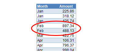
Oh dear. Not so good. The reason is simple. When selecting “Feb”, the number of Occurrences is two [2]. However,

IF(Data[Month]=Month_Selected,Data[Amount])

creates the list

{FALSE, FALSE, 897.34, 488.13, FALSE, FALSE, …}

SEQUENCE (Occurrences) creates the result {1, 2}, so INDEX will pick the first two items in the above list, which are both FALSE. It works for “Jan” as the first three values are for “Jan” – but not for any other month.  Thus, we need to add in a function that reorders our results so that the non-FALSE values will always occur first in the derived list. SORT is one such function:

=INDEX(SORT(IF(Data[Month]=Month_Selected, Data[Amount])), SEQUENCE(Occurrences))

This will have the desired effect of moving the non-FALSE values into the top positions of the list:

{488.13, 897.34, FALSE, FALSE, FALSE, FALSE, …}

Therefore, the results will display as follows:

This will differ from the aforementioned FILTER function as this will display the Amounts in the order they are encountered in the Data Table, viz.

This is because of the source data:

Word to the Wise

INDEX SEQUENCE is probably not the most essential combination in Excel, but it is frequently used to achieve results similar to those presented above. Filtering may generate similar results

The Top 10 continues next month.