Top 12 Excel Combinations: 10. SUMPRODUCT SIGN (Multiple Conditions with OR)

For 2024, I thought I would count down a very subjective “Top 12” of Excel function combinations. And this month’s offering makes it very clear that this is a highly subjective list. If you don’t like this month’s suggestion, feel free to email your views to someonewhocares@sumproduct.com.

Starting our Top 10, the 10th of 12, is a combination which avoids writing extremely horrendous formulae on occasion. This month’s couplet introduces SUMPRODUCT SIGN into my honours list.

Often in financial modelling you have to work with multiple criteria and the “OR situation” (i.e. I don’t need all criteria specified to hold) can provide consternation.

Excel has two functions that deal with OR:

1. OR(Condition_1,Condition_2,…) checks to see if any of the logical conditions specified are TRUE. As long as at least one condition is TRUE, OR will be TRUE also
2. XOR(Condition_1,Condition_2,…) checks to see if each of the logical conditions specified are TRUE. As long as at one and only one condition is TRUE, XOR will be TRUE also. This is often referred to as “exclusive or”.

XOR is a more recent function (first being introduced in Excel 2013) which is why many are not aware of it. If you are evaluating multiple conditions with OR, for non-Excel 365 and older versions of Excel you needed SUMPRODUCT.

At first glance, SUMPRODUCT(vector1, vector2, ...) appears quite humble. Consider the following sales report:

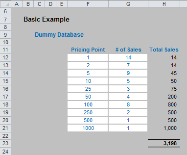
The sales in column H are simply the product of columns F and G, e.g. the formula in cell H12 is simply =F12*G12. Then, to calculate the entire amount cell H23 sums column H. This could all be performed much quicker using the following formula:

=SUMPRODUCT(F12:F21,G12:G21)

i.e. SUMPRODUCT does exactly what it says on the tin: it sums the individual products.

Where SUMPRODUCT comes into its own is when dealing with multiple criteria. This is done by considering the properties of TRUE and FALSE in Excel, namely:

• TRUE*number = number (e.g. TRUE*7 = 7); and
• FALSE*number = 0 (e.g. FALSE*7=0).

Consider the following example:

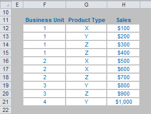
we can test columns F and G to check whether they equal our required values. SUMPRODUCT could be used as follows to sum only sales made by Business Unit 1 for Product Z, viz.

=SUMPRODUCT((F12:F21=1)*(G12:G21=”Z”)*H12:H21).

For the purposes of this calculation, (F12:F21=1) replaces the contents of cells F12:F21 with either TRUE or FALSE depending on whether the value contained in each cell equals 1 or not. The brackets are required to force Excel to compute this first before cross-multiplying.

Similarly, (G12:G21=”Z”) replaces the contents of cells G12:G21 with either TRUE or FALSE depending on whether the value “Z” is contained in each cell.

Therefore, the only time cells H12:H21 will be summed is when the corresponding cell in the arrays F12:F21 and G12:G21 are both TRUE, then you will get TRUE*TRUE*number, which equals the said number.

Notice that SUMPRODUCT is not an array formula (i.e. you do not use CTRL + SHIFT + ENTER), but it is an array function, so again it can use a lot of memory making the calculation speed of the file slow down.

But what if we only need one of these two criteria to be TRUE..?

Let us imagine we run a car sales company with four divisions: North, South, East and West. Further, we only sell two types of car: the Mercudi and the Lexota. This month’s attached Excel file may be used to follow this illustration:

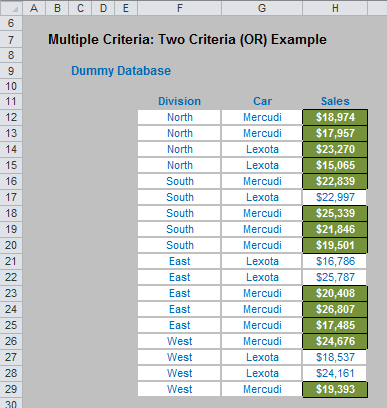
You are the General Manager responsible for the North Division and Mercudi sales. Each month you have to provide a report summarising the total sales you are responsible for. This requires analysis of multiple criteria, but it is an OR, rather than an AND, situation.

We need to include sales of North Division and sales of Mercudi. However, if we do it this simply sales of Mercudi made by the North Division will be double counted:

If we specify the criteria in the spreadsheet as follows:

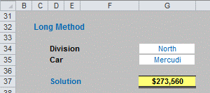
The formula in this instance would be:

=SUMPRODUCT((F12:F29=G34)*H12:H29)

+SUMPRODUCT((G12:G29=G35)*H12:H29)

-SUMPRODUCT((F12:F29=G34)*(G12:G29=G35)*H12:H29)

However, there’s a simpler approach…

Not many know this obscure but useful little Excel function. SIGN(number) is:

• 1 if number is positive
• 0 if number is zero
• -1 if number is negative.

It’s only when you start combining this function with SUMPRODUCT do you realise how useful it can be. For example, in our scenario above, consider the following formula:

=SUMPRODUCT(SIGN((F12:F29=G34)+(G12:G29=G35))*H12:H29)

Inside the nested SIGN function, there are two criteria:

1. whether the Division is North (F12:F29=G34); and
2. whether the car sold is the Mercudi (G12:G29=G35).

Each criterion will either be TRUE (1) or FALSE (0), so the possible values inside the SIGN function are zero (neither criteria satisfied), one (only one criterion satisfied) or two (both criteria satisfied). If neither criteria is true, SIGN will return a value of zero; if one or more criteria is true, SIGN will return a value of one and hence sum the relevant values in column H. This is precisely what is required.

With more criteria considered, the simplicity of SUMPRODUCT(SIGN) becomes even more pronounced. For example, this month’s attached Excel file considers three and four criteria, as well as two. For the sake of brevity here, I will jump straight to the four criteria scenario.

In this example, having been a very successful General Manager, you have acquired greater responsibility: not only do you remain responsible for the North Division and Mercudi sales, but you are now mentor to salesperson Alice and for trying to push credit (finance) sales.

As before, each month you have to provide a report summarising the total sales you are responsible for, which now considers four criteria: division, car, salesperson and finance:

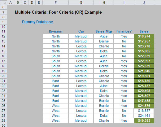
If we specify the criteria in the spreadsheet as follows:

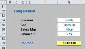
The “long” formula in this instance which would ensure the overlaps are not counted more than once would be:

=SUMPRODUCT((F12:F29=G34)*J12:J29)

+SUMPRODUCT((G12:G29=G35)*J12:J29

+SUMPRODUCT((H12:H29=G36)*J12:J29)

+SUMPRODUCT((I12:I29=G37)*J12:J29)

-SUMPRODUCT((F12:F29=G34)*(G12:G29=G35)*J12:J29)

-SUMPRODUCT((F12:F29=G34)*(H12:H29=G36)*J12:J29)

-SUMPRODUCT((F12:F29=G34)*(I12:I29=G37)*J12:J29)

-SUMPRODUCT((G12:G29=G35)*(H12:H29=G36)*J12:J29)

-SUMPRODUCT((G12:G29=G35)*(I12:I29=G37)*J12:J29)

-SUMPRODUCT((H12:H29=G36)*(I12:I29=G37)*J12:J29)

+SUMPRODUCT((F12:F29=G34)*(G12:G29=G35)*(H12:H29=G36)*J12:J29)

+SUMPRODUCT((F12:F29=G34)*(G12:G29=G35)*(I12:I29=G37)*J12:J29)

+SUMPRODUCT((F12:F29=G34)*(H12:H29=G36)*(I12:I29=G37)*J12:J29)

+SUMPRODUCT((G12:G29=G35)*(H12:H29=G36)*(I12:I29=G37)*J12:J29)

-SUMPRODUCT((F12:F29=G34)*(G12:G29=G35)

*(H12:H29=G36)*(I12:I29=G37)*J12:J29)

It’s just so pretty. PhD’s are available for all those of you who can follow this formula in a heartbeat. Surely you would you use the SUMPRODUCT(SIGN) variant (below) instead?

=SUMPRODUCT(SIGN((F12:F29=G34)+(G12:G29=G35)

+(H12:H29=G36)+(I12:I29=G37))*J12:J29)

Erm, maybe because it’s shorter, easier to read, less memory intensive, takes less time to calculate, is less prone to reference errors, has fewer opportunities for logic errors, …

Word to the Wise

For those living and breathing Office 365 and dynamic arrays, you may now be jumping up and down arguing SUMPRODUCT is superfluous. Indeed, in the brave new world, the last formula could be replaced with

=SUM(SIGN((F12:F29=G34)+(G12:G29=G35)

+(H12:H29=G36)+(I12:I29=G37))*J12:J29)

However, there are two reasons why I used SUMPRODUCT:

1. The formulae presented above work in all versions of Excel
2. Our company name is SUMPRODUCT!

The Top 10 continues next month.