In recent months, there has been a lot of hype about the new GROUPBY and PIVOTBY functions in Excel. As of late September 2024, these functions are now “generally available”, so they will be coming to all Excel 365 users at their next update cycle.

As we has already covered those functions in a previous post (Excel’s new functions might change data analysis forever), we are not looking at those functions in detail. Instead, we are answering just one question, which I know many users will be thinking: how can we use slicers with these new functions?

We introduced similar concept in a previous post (The truth about the FILTER function), but in this post, we are going deep to really understand how it works.

I recommend downloading and looking at the example file to see how this solution comes together.

Table slicers

Tables are a critical Excel feature, they allow us to hold data in a structured format.

Here is the Table we are using in this post – it is called Sales.

One key aspect of Tables is the ability to use slicers. All we need to do, is select a cell in the Table and click Insert > Slicer (or Table Analyze > Insert Slicer) from the ribbon.

This leads to the Insert Slicers dialog box, where we can select which columns we want to create slicers for.

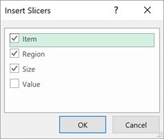
In our example, I have created slicers for the Item, Region and Size columns.

Once created, clicking the slicer buttons filters the Table. The rows for the slicer selected values are displayed and the unselected values are hidden.

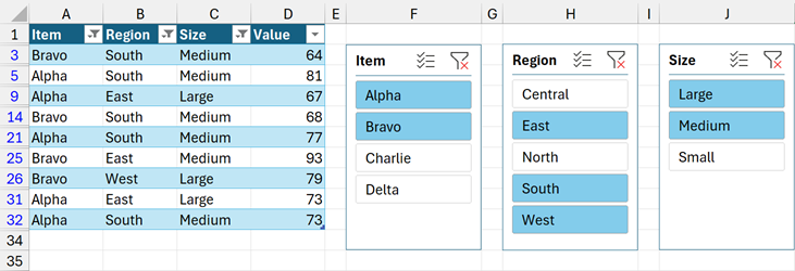
Even though a Table is a separate data object, it lives on the grid. As a result, for any items not selected, the entire row of the worksheet is hidden. Therefore, to implement the techniques in this post it is best to place the Table and formulas on separate sheets.

SUBTOTAL function

SUBTOTAL is commonly used for working with hidden and filtered cells. This is because one of SUBTOTAL’s superpowers is the ability to exclude hidden rows from a calculation.

Normally, we use SUBTOTAL to perform aggregation calculations over a range. The function_num argument determines the type of aggregation we wish to perform.

For example, to calculate the number of visible rows in a Table column we might use SUBTOTAL as follows:

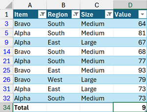
The function in cell D34 is:

=SUBTOTAL(3,Sales[Value])

• 3 is the function number for COUNTA (which counts all populated cells).
• Sales[Value] is the range to calculate on.

This is telling us there are 9 visible rows in the Table.

But what would happen if we applied the same calculation to each row of a Table, instead of the column of a Table? SUBTOTAL would calculate each visible row as 1 and each hidden row as 0.

There is a big issue with SUBTOTAL. We want SUBTOTAL to calculate for each row, but SUBTOTAL is an aggregation function which returns a single value. Therefore, it can’t calculate for every row. This is where a function combination like BYROW/LAMBDA comes in.

The BYROW/LAMBDA combination forces a calculation to occur row by row. So, by including SUBTOTAL inside a BYROW/LAMBDA, it causes SUBTOTAL to calculate once for each row.

For example, we could use the following formula:

=BYROW(Sales[Value],LAMBDA(r,SUBTOTAL(3,r)))

• BYROW is a function which calculates once for each row.
• Sales[Value] is the range of cell to calculate over.
• LAMBDA(r,_______) creates a variable called r which represents the values in each row of the range.
• SUBTOTAL(3,r) performs a COUNTA calculation on each r (ie, on each row in the Sales[Value] range).

The result would be an array of 1’s or 0’s. The 1’s represent each row which is visible; 0’s represent each row which is hidden.

FILTER, GROUPBY and PIVOTBY functions

The FILTER, GROUPBY and PIVOTBY functions include the filter_array (for GROUPBY and PIVOTBY) and include (for FILTER) arguments.

These arguments determine which rows of the source data are included/excluded from the calculation. So for each row of the data there must be a corresponding TRUE/FALSE value. Only the rows with TRUE results are included in the result.

We know that, in Excel, 0’s are treated as FALSE and 1’s are treated as TRUE. Therefore, we can use the result of the BYROW/LAMBDA/SUBTOTAL combination created above for the TRUE/FALSE values.

Bringing it all together.

Let’s bring all this knowledge together.

We have already been introduced to the Sales table. Now, let’s introduce a few more elements.

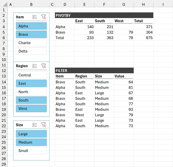
We have a separate worksheet called Report. On this worksheet we have slicers for the Item, Region and Size columns of the Sales table.

This worksheet includes only two formulas in cells D3 and D14.

The formula in cell D3 includes the PIVOTBY function:

=PIVOTBY(Sales[Item],Sales[Region],Sales[Value],SUM,,,,,,
BYROW(Sales[Value],LAMBDA(r,SUBTOTAL(3,r))))

• Sales[Item] is the values to include in the rows.
• Sales[Region] is the values to include in the columns.
• Sales[Value] is the values to include in the body of the calculation.
• SUM is the calculation to perform on the Sales[Value].
• BYROW(Sales[Value],LAMBDA(r,SUBTOTAL(3,r)))) ensures only the values selected by the slicer are included in the result.

Remember to look at our previous post to understand all the options of the PIVOTBY function.

The formula in cell D14 is a FILTER function:

=FILTER(Sales,BYROW(Sales[Value],LAMBDA(r,SUBTOTAL(3,r))))

• Sales is the name of the Table.
• BYROW(Sales[Value],LAMBDA(r,SUBTOTAL(3,r)))) ensures only the values selected by the slicer are included in the result.

Using these two formulas, we have a cross-tab report (created by PIVOTBY) and a detailed list (created by FILTER).

Clicking the slicer buttons:

1. causes the table to filter,
2. which causes BYROW/LAMBDA/SUBTOTAL to recalculate,
3. which causes PIVOTBY and FILTER the recalculate,
4. which spills the values on the grid

So through the calculation chain, we are able to use slicers with these new formulas.

Conclusion

The latest Excel functions give us a lot of reporting flexibility. By using a BYROW/LAMBDA/SUBTOTAL combination we can use slicers to take these new functions even further.

• Download an example file to see the solution in action.