Sometimes when I run training courses, I realise that we are all in danger of using the bulldozer in a china shop approach to solving problems in Excel. We can all be guilty of using Power Pivot, Power Query, LET, LAMBDA and other powerful functions and features to solve problems where simpler, older tools will do the trick. I’d like to illustrate one such instance below.

Imagine you are in charge of quarterly reporting and you are required to analyse quarterly actual performance actuals against budgeted data.  You might have data such as the following:

Please review the attached Excel example file for the scenarios I use.

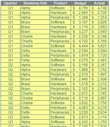
I have called this (CTRL + T) Table Calc_Fields_Source. It contains Budget and Actual sales data broken down by Quarter, Business Unit and Product. I want to analyse this in a PivotTable, together with the variance.

I could create another column in the Table:

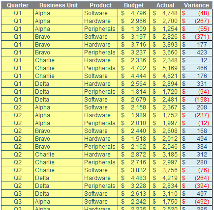
Here, the formula for the Variance is given by

=[@Actual]-[@Budget]

which uses Structured Referencing, the coding language of Tables (the formula literally means subtract the Budget data on this row from the Actual data on this row).

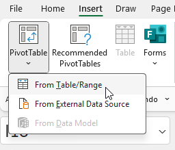
The problem is if I have a million records I have just added a million calculations, which will lead to a bloated file size and extra memory usage. The fact is I don’t need the Variance column. Instead, I will create a PivotTable by selecting the Table and then use Insert -> PivotTable -> From Table / Range (ALT + N + V + T), viz:

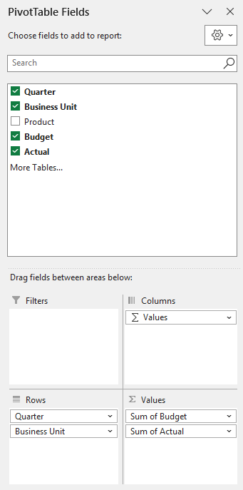
Using the default settings for PivotTables, I can report by Quarter and Business Unit in the Rows area of the PivotTable, with Budget and Actual in the Values area:

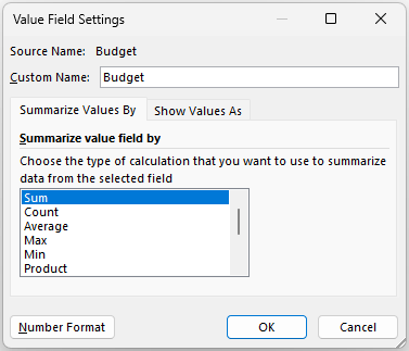
By clicking on the ‘Sum of Budget’ and ‘Sum of Actual’ items, I can access the shortcut menu and from the ‘Value Field Settings’ change the names to ‘Budget ‘ and ‘Actual ‘. Note the trailing space: the names cannot be the field names from the Table (this is not allowed in Excel), so adding a space makes for a good “cheat”. Here is ‘Budget ‘ as an example:

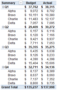
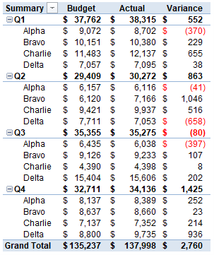
Relabelling ‘Row Labels’ as ‘Summary’ in the top left-hand corner of the PivotTable will render the following result:

So how do we get the Variance? Simply click inside the PivotTable to activate the context specific tabs in the Ribbon. From the ‘PivotTable Analyze’ tab, click on the ‘Fields, Items, & Sets’ button and choose ‘Calculated Field…’.

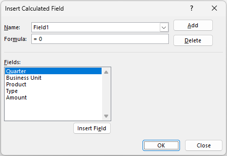
This gives rise to the ‘Calculated Field’ dialog:

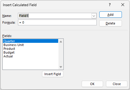
This dialog uses a programming language called Multidimensional Expression for Cubes – or MDX for short. Its name is probably more complicated than its syntax. For example, to create my Variance calculated field, I just need to do the following:

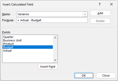
All you have to do is type in the ‘Name:’ and in the ‘Formula:’ section you can select from the Fields list for simple calculations in seconds. I just click OK, and with a little formatting and renaming the field ‘Variance ‘ (with a space again), I can get readily create the following PivotTable:

There is no need for Power Pivot or the additional column / field in the source table: I merely employ a calculated field. This is simply the formulaic manipulation of one or more fields.  Simple!

There are quite a few who are aware of this feature in PivotTables, but I suspect fewer are aware of calculated items. These do not seem to be so common and / or popular.  Therefore, let me show you a second scenario where you might require such a feature.

Let’s consider the second example in the same attached Excel example file. Again, we are still required to analyse quarterly actual performance actuals against budgeted data. However, this time our source data is slightly different:

Let’s call this (CTRL + T) Table Calc_Items_Source. Do you see the difference between this and the first Table? Here, we do not have a Budget and an Actual column. In this case, we have an Amount field and a separate field that ascribes whether the value is a Budget or an Actual figure. This is going to cause us problems. But not insurmountable ones!

As before, I will create a PivotTable by selecting the Table and then use Insert -> PivotTable -> From Table / Range (ALT + N + V + T), viz:

Using the default settings for PivotTables, I can again report by Quarter and Business Unit in the Rows area of the PivotTable. After that, things change:

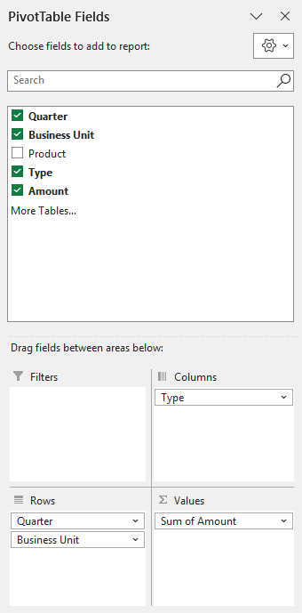
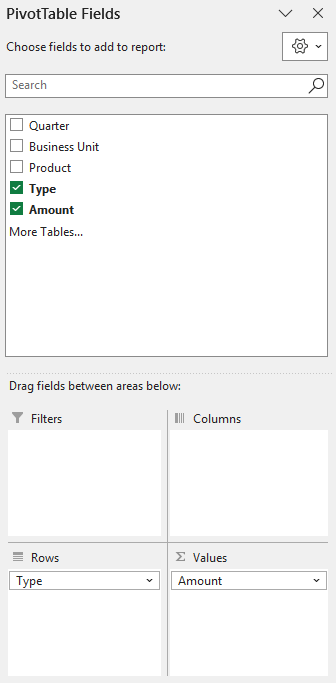
On this occasion, I have to put the Type filed into the Columns area and Amount (which becomes ‘Sum of Amount’) into the Values area of the ‘PivotTable Fields’ pane.

By clicking on the ‘Sum of Actual’, I can access the shortcut menu and from the ‘Value Field Settings’ change the name to ‘Actual ‘ with the trailing space once more. Relabelling ‘Row Labels’ and ‘Column Labels’ in the PivotTable will yield the following result:

The Type field has been split into two categories, Actual and Budget, together with a Grand Total, which I shall remove from the PivotTable. I need to calculate the Variance once more. Therefore, I replicate the steps from last time and click inside the PivotTable to activate the context specific tabs in the Ribbon.

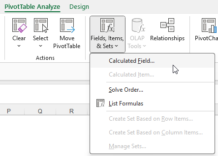
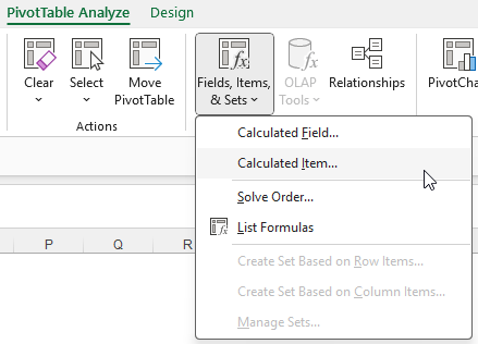
From the ‘PivotTable Analyze’ tab, I then click on the ‘Fields, Items, & Sets’ button. At this stage one of two things will happen: in the resulting menu, the second item, ‘Calculated Item…’ will either be greyed out (as in the image below) or else will be visible. We will resolve this shortly, but first we will click on ‘Calculated Field…’ as before:

This gives rise to the following dialog:

Uh oh. There is no Actual or Budget field.

That’s right: Actual and Budget are categories of the Type field. They are not fields in their own right. ‘Calculated Field’ will not work for us in this instance. We need ‘Calculated Item…”. 

And that’s where we might hit a problem.

First, check which cell you have clicked on in the PivotTable. You must ensure you are in the Columns part of the PivotTable; you must not have selected a value or row item. If you are certain you have positioned yourself in a column item and ‘Calculated Item…’ remains greyed out, this is probably because a calculated item in some versions of Excel may only be calculated on fields in the Rows area of the ‘PivotTable Fields’ pane. In this case, and this case only, it’s time to rearrange our PivotTable:

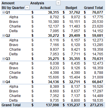
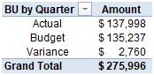
I remove the fields (Quarter and ‘Business Unit’) from the Rows area and drag Type into this area. That’s right, dear reader: I’m reverting to Type (sigh – Ed.). Our PivotTable now looks like this:

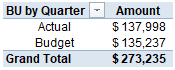
I accept the label ‘BU by Quarter’ is wrong, but no matter, this is only a temporary layout of the PivotTable whilst we create the calculated item. With Type in the correct area, I ensure I have clicked in the left-hand column of the PivotTable to activate the context specific tabs in the Ribbon. From the ‘PivotTable Analyze’ tab, I then click on the ‘Fields, Items, & Sets’ button:

‘Calculated Item…’ will only be available if I have clicked in the Type section of the PivotTable. Only items in the Rows area of the ‘PivotTable Fields’ pane may be used for creating a calculated item. Once I click on this menu item, I get the following ‘Calculated Item’ dialog:

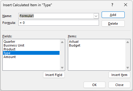
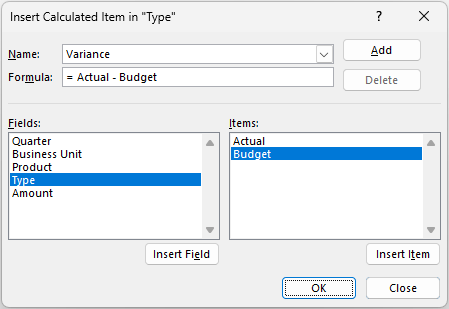
This is similar to the ‘Calculated Fields’ dialog, except here we create formulae out of items in a particular field. Here, I will select Type and use Actual and Budget items in my formula as follows:

Clicking OK, I get the following result in the PivotTable:

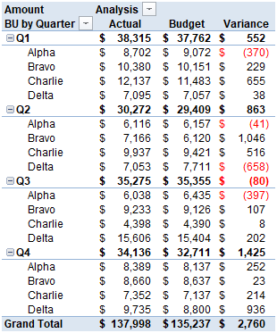
I now reorder the PivotTable as previously in the ‘PivotTable Field’ pane:

Of course, if ‘Calculated Item…’ was not greyed out, you simply needed to define Variance as above without manipulating the positioning of fields in the PivotTable.

In either case, removing the Grand Total for rows, together with a little formatting, I can create the following PivotTable:

It’s a crafty, little-known trick but it generates what we want without having to undertake more complex manipulation in some cases. I think people don’t employ it as you have to move fields around on the PivotTable and then move them back for some versions of Excel. However, it’s well worth knowing as this scenario occurs in reality time and time again.

Word to the Wise

Calculated items are not as frequently used or as well understood as their calculated field counterparts. It should be remembered they can only be applied to fields in the Rows area (or Columns area for some versions of Excel) of the ‘PivotTable Fields’ pane. Any field used to generate a calculated item may not be added to the PivotTable a second time, including being used as a filter.

Furthermore, if you use too many calculated items in your Excel file, it can cause calculations to slow down – so use this trick sparingly!