Sometimes, you wish to sum values in an array based upon their categories.  The world is moving on with dynamic arrays, and this month, I thought I would show you how you could summarise results that will extend in multiple dimensions.

• Download the example file

Please note I have used random numbers for inputs, so do note that the values keep changing between the screenshots – but at least this highlights the solution will be both robust and flexible!

Imagine you had the following input data, where you have the sales of products A, B and C over 10 periods, and you wanted to summarise it as follows:

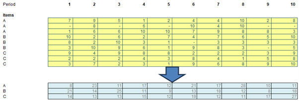
There are several issues:

• you wish to create a unique list of products
• you want to summarise it over the multiple periods, yet condense the rows
• you want the range to extend automatically if there are more products and / or more periods.

For those who read my articles regularly you will know I am a great fan of SUMPRODUCT (so much so that our company was named after this infamous Excel function).  By multiplying output category and period by the input category and period vectors we can get our answer for each individual output cell.  Using the example file, I might try the following:

=SUMPRODUCT($F$16:$O$24*($D33=$D$16#)*(F$13=$F$13#))

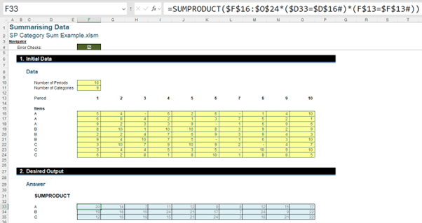
Unfortunately, this method doesn’t spill and therefore doesn’t satisfy our criteria.

You might consider using the SUMIFS function to sum each column by category.  This requires a minimum of three arguments:

=SUMIFS(sum_range, criteria_range1, criteria1, …)

The sum_range is the range of cells to sum, the criteria_range1 is the first range being tested using criteria1 and criteria1 is the criteria being used to filter criteria_range1.  You can add as many criteria and criteria ranges as you like.

In this case, if we wanted to get a category sum for an individual row, we could use SUMIF on the row.  The criteria range would be the list of items for the array, whilst the criteria would be the specific item we are filtering for.

Some people may be tempted to apply SUMIFS over the whole array and filter by the period as well to try and make the whole array dynamic.  This doesn’t work as SUMIFS only works in one dimension.

My solution utilises the MMULT function, which is used to multiply two matrices together.  Firstly, a quick refresher on how matrix multiplication works.

The output of two matrices multiplied is the height of the first matrix and the width of the second matrix.  The width of the first matrix and the height of the second matrix should be equal.  The cell outputs are found by multiplying the values in the corresponding row from the first matrix and column from the second matrix and adding the products.  For example, for the bottom left output, you take the second row of the first matrix and the first column of the second matrix: (1 x 4) + (1 x 4) + (5 x 1) = 13.

To start, we need to create a helper array. First, we use the TRANSPOSE function on our large categories list to turn it horizontal.  By equating this to our unique categories list we can create a helper array of 1’s and 0’s.

(D33#=TRANSPOSE(D16#))*1

This helper array links each item row to their category. We can actually put this inside the MMULT function and multiply it by the source array to find the total for each category and period.

=MMULT(N(D33#=TRANSPOSE(D16#)), F16#)

This takes each column and multiplies each value in the period by either one [1] if it’s in the category being checked or by zero [0] if it isn’t and adds them together, giving us just the total from that category and period.

Can you find a shorter solution?

Word to the Wise

Just for fun, another solution can be found using the SUBTOTAL function combined with OFFSET.  To be clear, this solution is longer and unnecessarily complex, but it’s also quirky and interesting so worth showing here.  The SUBTOTAL function can perform a range of tasks, in this case we will be using function 9 which allows us to SUM over a whole dynamic range – but unlike SUM, the calculation will spill rather than coerce.  This highlights there are inconsistencies in the Excel calculation engine!

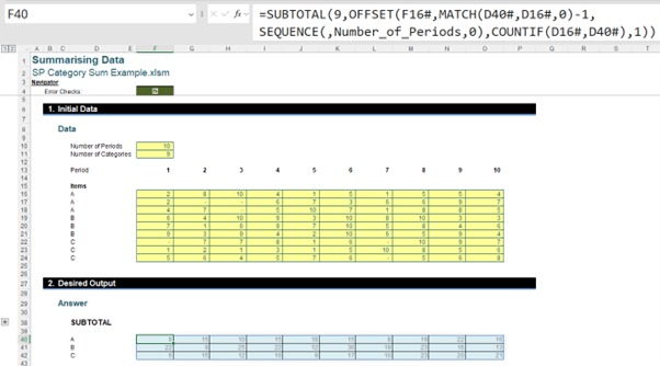
The formula I am using is:

=SUBTOTAL(9,OFFSET(F16#,MATCH(D40#,D16#,0)-
1,SEQUENCE(,Number_of_Periods,0),COUNTIF(D16#,D40#),1))

This looks intimidating so let me break it down. The MATCH function returns the row of the first appearance of each letter in the matrix. Therefore, for the above, it would be {1;4;7}.  It’s subtracted by one [1] because OFFSET already starts pointing to the first row.  The COUNTIF function returns the number of rows corresponding to each letter, in this case, it is simply {3;3;3}.  The SEQUENCE function returns a list of integers growing from one [1] to the number of periods.

When we put all of this into the OFFSET function this returns three [3] times the number of periods as an array of arrays, with each position in the array containing the values that correspond to that period and that category, e.g. the top left contains the array {1;7;7}. SUBTOTAL allows us to sum up these internal arrays and returns a spilled array of the summed values.