Introduction

Spreadsheets, and technology in general for that matter, can be fantastic. Until that is, things don’t go as expected. It’s all too easy for an entire month’s productivity gains to be lost when sorting out a single spreadsheet problem. In this series, we will be look at some examples of Excel not doing what we expect and at how to deal with the problems.

So far, we have looked at the basic problem of our numbers not adding up and looked at solving the problem using Excel’s ROUND() function before warning about the use of the Precision as Displayed option. This time we are going to examine the issues of ranges that don’t include all the cells that they should.

When 42 isn’t the answer

If you looked carefully enough at the penultimate screenshot in the first article, you might have noticed four values of 21 appearing to add up to 42:

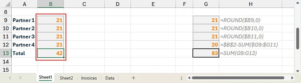
Our example involved increasing the number of partners receiving a share of our profit from 2 to 4. To do this, we inserted two complete rows into our spreadsheet above our Total row, before extending our formula into the two new rows. Because we inserted our rows underneath, rather than in the middle of, our existing range of cells, our SUM() range didn’t automatically expand to include the new rows.

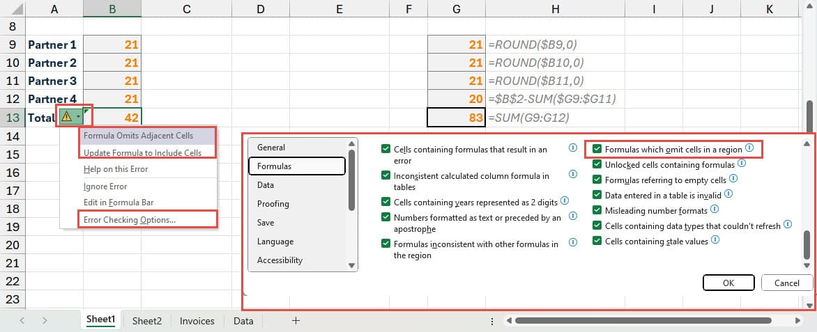
This is such a common problem that Excel has a specific error checking rule to add a warning to cells that contain: ‘Formulas which omit cells in a region’. If the values in our four cells had just been typed in values of 21, our Total should display a background error checking indicator. By default, this would be a green triangle in the top left-hand corner of the cell. Clicking on the warning icon that appears when we select the cell, would then display an explanation of why a warning was being displayed, and offer to correct the problem:

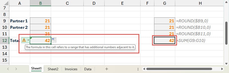
Useful as the error checking might be, it should not be relied upon to highlight all errors that can occur. For example, as we have already seen, if we are adding up cells that contain formulas rather than values, setting an incomplete range of cells will not generate our warning. Here, we have values in column B and formulas in column G. We have inserted a row immediately above our Total row and copied the value or formula from the row above into cells B11 and G11. Our Total cell in column B displays an error check warning, but no warning is shown in column G because the range has additional formula cells, rather than additional numbers, adjacent to it:

Tables

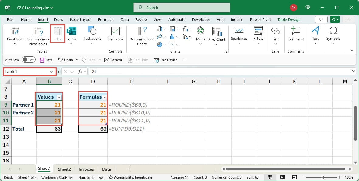
One way to reduce the likelihood of incorrectly omitting cells from a range is to use Excel Tables. If the range you are referring to is a Table column, then your formula should automatically adjust to include new cells added immediately below the existing range of cells, whether those cells contain values or formulas.

This time, we have added a heading in cell B8 before selecting cells B8:B10 and using the Insert Ribbon tab, Tables group, Tables command to turn the three cells into a Table. We could use the Control+t keyboard shortcut instead. Excel automatically gives our Table the name Table1, but we could give the Table a more informative name using the Table Design Ribbon tab. We then repeat the process in the equivalent cells in column D. Now, when we insert our row immediately above our Total and copy our cell values and formulas from row 10 down to row 11, the ranges in both of our total cells should automatically adjust to include the new cells:

Next time

In the next part of this series, we will try and answer the age-old question: when is a number not a number?

Additional resources

You can explore all aspects of Excel, including many articles on the advantages of using Excel Tables, in the ICAEW archive:

• Excel archive