Introduction

Spreadsheets, and technology in general for that matter, can be fantastic. Until that is, things don’t go as expected. It’s all too easy for an entire month’s productivity gains to be lost when sorting out a single spreadsheet problem. In this series, we will be look at some examples of Excel not doing what we expect and at how to deal with the problems.

So far, we have looked at the basic problem of our numbers not adding up and looked at solving the problem using Excel’s ROUND() function before warning about the use of the Precision as Displayed option and examining the issues of ranges that don’t include all the cells that they should. This time we will look at another cause of mysterious maths issues – numbers that are not always numbers (but are sometimes…)

When 63 isn’t the answer either

The last article’s investigation of incomplete cell ranges started with 4 cells, each containing the value 21, seeming to add up to 42. This time, our 4 cells seem to add up to 63:

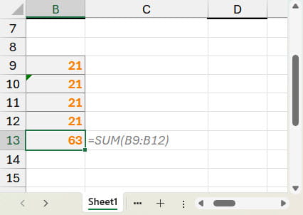
If we look at our SUM() formula we can see that, this time we have used the correct range of cells. In fact, the issue is with the value in cell B10. It might look like the number 21, but it has been entered as a text value, preceded by an apostrophe. We have had to do a little more to make our text look like a number. In order to prevent the text value from looking different to our ‘proper’ numbers we need to change the alignment from the default left for text, to the right-alignment used as the default for numbers. Also, another of the Excel error-checking options that we featured last time, will highlight a ‘Number Stored as Text’:

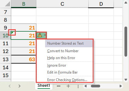
Although the error-check should normally highlight the issue with an indicator in the top left-hand corner of the cell, individual types of error check or error-checking in general can be turned off, or the error-check for specific cells can be ignored.

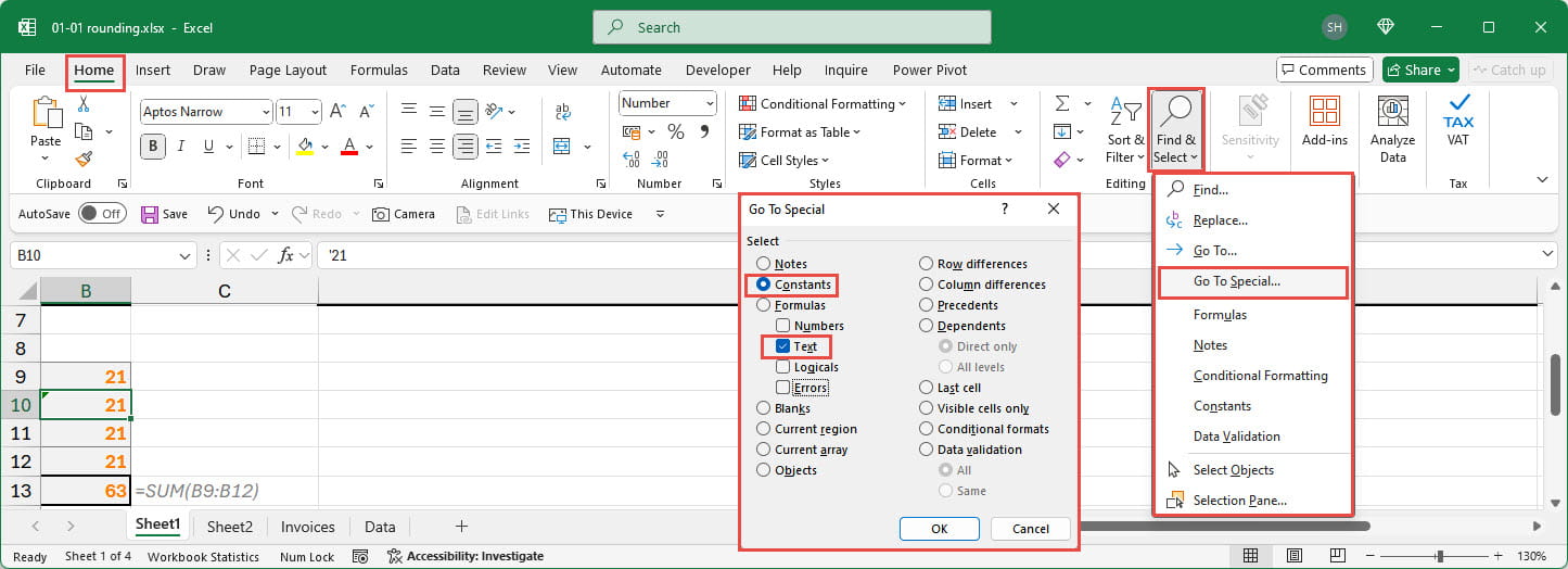
If we do suspect that some figures have been entered as text, there is another way to identify affected cells. The Home Ribbon tab, Editing Group, Find & Select, Go To Special dialog includes an option to select Constants, and then Text. If we were to select our range of cells, this will select our ’21 cell:

May the force be with you

Just before we replace our text 21 with a proper number, we will create our total using a different formula. Rather than using SUM() we will just add our four cells using the plus operator:

=B9+B10+B11+B12

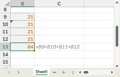
Perhaps surprisingly, our formula returns the value of 84, despite the inclusion of a cell that contains text. This gives us the surprising result that the use of the SUM() function to add 4 cells gives a different result from adding the same four cells using the plus operator. This is by design. The SUM() function is designed to ignore text values in a range and add up the numeric values that remain. In contrast, using an arithmetic operator forces (or coerces) text values to be treated as numbers, as long as the text value only contains numeric characters. In effect, when we specifically use an arithmetic operator such as plus, Excel realises that we want to work with numbers and so it does its best to cooperate by ‘coercing’ text that only contains numeric characters to become a number.

May the FALSE be zero

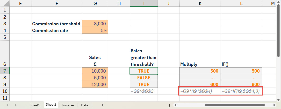
In fact, coercion isn’t just restricted to text. It also works with Boolean (TRUE/FALSE) values. A value of TRUE is treated as the number 1 whereas FALSE is 0. This allows the use of the multiply operator to be used as an alternative to the IF() function. Multiplying a value by a TRUE value will return the value, multiplying it by a FALSE value will return Zero:

Next time

In the next part of this series, we will examine the use of the IF() function in more detail.

Additional resources

You can explore all aspects of Excel in the ICAEW archive:

• Excel archive