REDUCE is one of those advanced functions which intimidate many Excel users. The goal of this post is to help you understand how REDUCE works and provide some real-world examples where it can achieve the impossible.

We have looked at REDUCE in previous posts, which you can find here:

• Excel Tips & Tricks #474 - How to REDUCE repetitive calculations to a single step
• Solving the array of arrays issue

Example 1: Basic example

Microsoft’s definition of REDUCE is:

“Reduces an array to an accumulated value by applying a LAMBDA to each value and returning the total value in the accumulator.”

I know, I know… that makes no sense whatsoever! So, let’s explain this with a basic example.

Scenario

Let’s suggest we have a product with a standard sale price of £1,000.

There are various discounts available for a specific customer: 

• Spring Sale Discount - 20% off
• Loyalty Club Discount - 10% off
• Supplier Promotion Discount - 15% off

How much is the final price?

If each discount is applied to the previously discounted price, then the saving is 38.8%; leaving the final price as £612.

• £1,000 less 20% discount = £800
• £800 less 10% discount = £720
• £720 less 15% discount = £612

We can calculate that in Excel as follows:

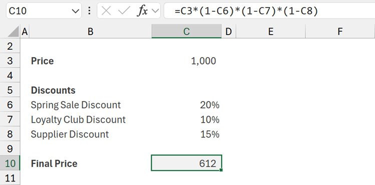
The formula in cell C10 is:

=C3*(1-C6)*(1-C7)*(1-C8)

We have 3 discounts available, and they are hardcoded into the formula. If we had more or less discounts we would need to change the formula each time.

Instead, we could use the REDUCE function.

The formula in cell C10 is now:

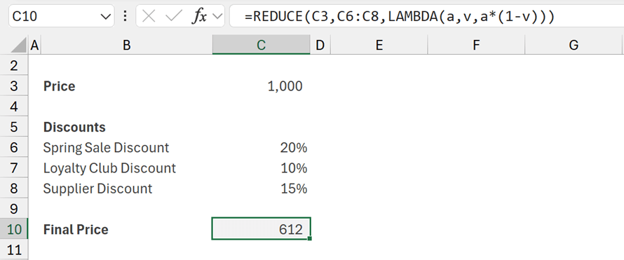
=REDUCE(C3,C6:C8,LAMBDA(a,v,a*(1-v)))

This probably looks confusing, so let’s break down this calculation.

Explanation

REDUCE has 3 arguments:

• Initial_value: The start value. Which for our example is £1,000 (the value in C3).
• Array: The list of items we want to use in the calculation. In our example it is the list of discount rates (the values in C6:C8).
• Function: The calculation we want to perform, which is the LAMBDA(a,v,a*(1-v)) section.

Let’s dig into the function argument to see what it is doing.

Using standard words, the calculation we want to perform is for each discount is:

Take the previous result and multiply it by one minus the current discount.

Which we could write as:

PreviousResult * ( 1 – CurrentDiscount )

We apply this calculation for each discount in the list. Whether we have 3 discounts or 100 discounts, the calculation remains the same. What changes is how many times we perform the calculation.

So, lets change the names slightly. Let’s change PreviousResult to a (which stands for accumulator) and CurrentDiscount to v (which stands for value). Our previous calculation…

PreviousResult * ( 1 – CurrentDiscount )

… now becomes…

a*(1–v)

Oh… wait… isn’t that our function:

LAMBDA(a,v,a*(1-v)))

Here the LAMBDA function is stating that:

• The Previous Result is called a
• The Current Discount is called v
• We want to perform a*(1-v) for every discount.

If we bring this together, it should now start to make sense.

• The initial_value declares the first value to use as a
• The array provides the list of v’s
• The function provides the calculation to perform using the a and v values.

Hopefully, you can now see what REDUCE does and how it works. It performs iterative calculations using the previous result as the basis for each calculation.

That’s the basic concept. Now let’s look at a few more examples.

Example 2: Find and replace text

In Excel, the SUBSTITUTE function can find and replace text.

Look at this function:

=SUBSTITUTE("ICAEW Excel Community","Community","Faculty")

In the text ICAEW Excel Community, the word Community would be replaced with Faculty.

The result would be: ICAEW Excel Faculty

That is a single find and replace calculation, but what if there were an unknown number of calculations? How could we handle that?

We would need to perform SUBSTITUTE multiple times, using the previous result as the basis for each calculation. The calculation could be stated as:

SUBSTITUTE(PreviousResult,CurrentFind,CurrentReplace)

Let’s turn to the REDUCE function once more.

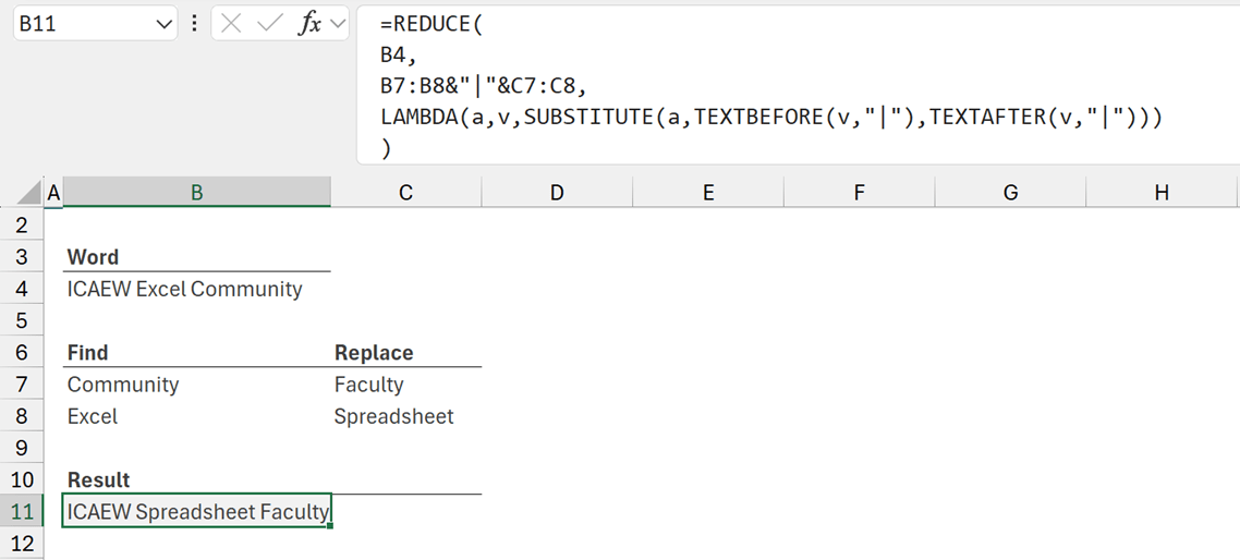
The formula in cell B11 is:

=REDUCE(
B4,
B7:B8&"|"&C7:C8,
LAMBDA(a,v,SUBSTITUTE(a,TEXTBEFORE(v,"|"),TEXTAFTER(v,"|"))
))

In words this calculation is:

• Start with ICAEW Excel Community.
• Take the previous result and replace Community with Faculty.
• Take the previous result and replace Excel with Spreadsheet.

The result is ICAEW Spreadsheet Faculty.

We have a complication with this example. We have two lists, the find list (B7:B8) and the replace list (C7:C8), but REDUCE only has one array argument.

We have solved this as follows:

• B7:B8&"|"&C7:C8 joins the find list and replace list into a single array with the values separated by the | symbol. (eg, Community|Faculty and Excel|Spreadsheet).
• The values are separated back into two by using TEXTBEFORE and TEXTAFTER.

You can find out more about TEXTBEFORE & TEXTAFTER in this article on text functions in Excel.

In this example we only have 2 pairs of items to find and replace, but it could be 100’s. Using REDUCE, the calculation can occur for as many items as are in the array.

In this example, we just have a single text value in B4. But what if we had multiple text values? That’s no problem, REDUCE returns a result for each of them.

The formula in cell B14 is:

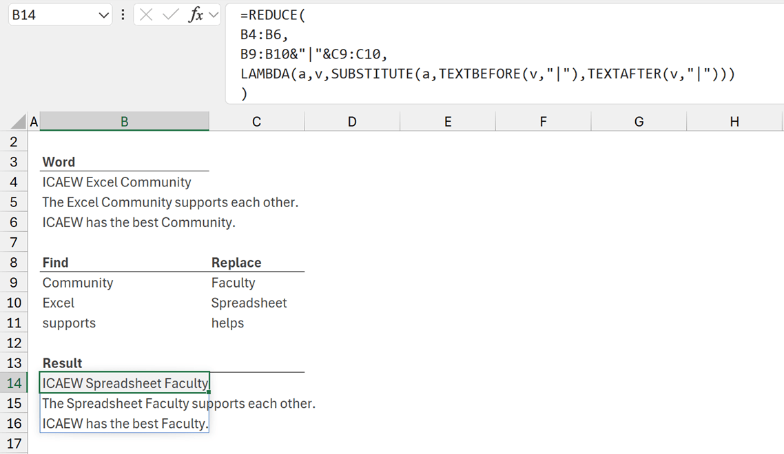
=REDUCE
( B4:B6,
B9:B10&"|"&C9:C10,
LAMBDA(a,v,SUBSTITUTE(a,TEXTBEFORE(v,"|"),TEXTAFTER(v,"|")))
)

B4:B6 contains multiple text strings. The find (B9:11) and replace (C9:C11) calculation is applied to all of them.

Example 3: Ragged arrays

Now let’s look at another example.

Let’s suggest we have a table including projects and the employees who worked on those projects. All we want is to display a column for each project with the employees listed.

So, let’s see how we can achieve this.

The formula in cell E3 is:

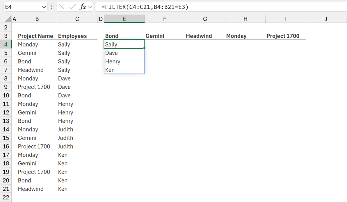
=TRANSPOSE(SORT(UNIQUE(B4:B23)))

Since project names could change this provides a dynamic unique sorted list of the projects.

The formula in cell E4 is:

=FILTER(C4:C23,B4:B23=E3)

This provides the list of employees for project Bond.

Since E3 is dynamic, we might think we could change E3 to E3# and all the values would populate. However, doing this returns the #VALUE! error. The reason for this are beyond the scope of this post. But let’s just say that FILTER doesn’t work like that.

So, how can we achieve this? Let’s take a look at REDUCE.

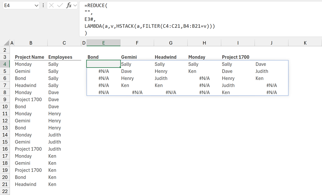
The formula in cell E4 is:

=REDUCE(
"",
E3#,
LAMBDA(a,v,HSTACK(a,FILTER(C4:C23,B4:B23=v)))
)

Let’s break this down.

E3# is the array for which we want to perform the calculation over. Each value in E3# is called v.

In the FILTER function we have used v instead of a fixed cell reference:

FILTER(C4:C23,B4:B23=v)

This means FILTER will calculate once for each project.

But we also want to stack each FILTER calculation onto the previous result to create a single value. To achieve this, we use HSTACK with the accumulator.

HSTACK(a,FILTER(C4:C23,B4:B23=v))

As FILTER calculates for each project, the result stacks onto the previous FILTER functions.

As shown in the image above, there are a few issues with our result, which we need to address.

Firstly, in this scenario, we don’t need an initial_value, we just want to stack the FILTER functions together. But, REDUCE must have an initial_value. Therefore, we have used an empty text string ( "" ) as the initial_value. We will remove this shortly.

Secondly, the results of each FILTER function is an array of varying sizes (2,3,4 or 5 rows). When HSTACK combines arrays of different sizes if fills the empty cells with #N/A.

To resolve these issues, we can add the DROP and IFERROR functions.

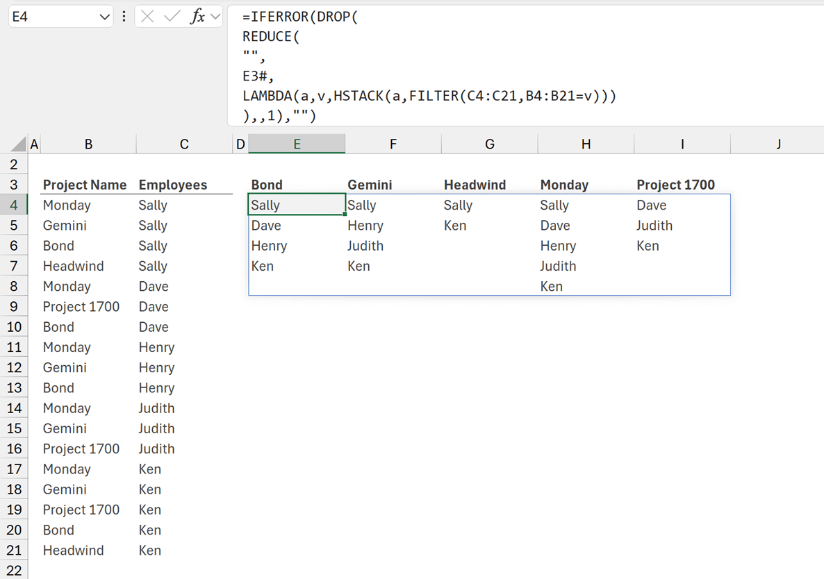
The formula in cell E4 is:

=IFERROR(DROP
( REDUCE("",
E3#,
LAMBDA(a,v,HSTACK(a,FILTER(C4:C21,B4:B21=v)))
),,1),"")

• DROP(_________,,1) removes the first column created by the initial_value.
• IFERROR(_________, "") replaces errors with empty text strings.

This provides us with exactly the result we want.

The combination of DROP, REDUCE, LAMBDA, HSTACK is very powerful. If we can calculate a single result, we can use this combination to perform many calculations and then combine them together into a single result.

NOTE: If values are stacked vertically VSTACK will be used in place of HSTACK. We will see this in the next example.

Example 4: Multiple TEXTSPLITs

TEXTSPLIT is one of Excel’s newer functions. As the name describes, it splits text.

The formula in cell B6 is:

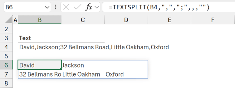
=TEXTSPLIT(B4,",",";",,,"")

This splits the text in B4, using a comma ( "," ) to separate columns, a semicolon ( ";" )to separate rows, and any missing values are padded with empty text stings ( "" ).

You can find out more about this in this article on TEXTSPLIT.

Unfortunately, if we we include multiple cells for the text, we only get the first column of values.

This is triggered by the array of arrays issue we covered in a previous article.

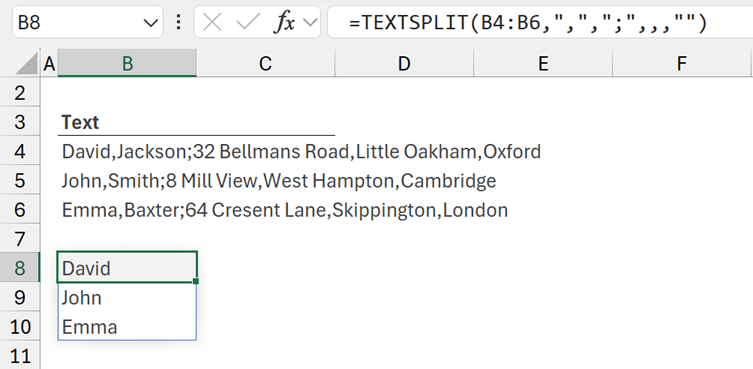
But don’t worry, we can use the REDUCE function once again to solve this.

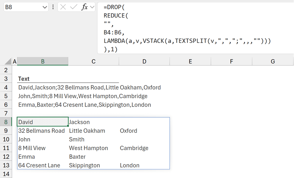
The formula in cell B8 is:

=DROP(
REDUCE(
"",
B4:B6,
LAMBDA(a,v,VSTACK(a,TEXTSPLIT(v,",",";",,,"")))
),1)

• The text to split is cells B4:B6. Each cell is called v.
• The TEXTSPLIT calculation is performed for each v, and VSTACKed into the previous result which is called a.
• REDUCE must have an initial_value, to use as the first a. For this we have used an empty text string ( "" )
• Since we don’t need the initial_value, we used DROP to remove the first row ( 1 ) from the result.

Conclusion

In this post, we have seen that REDUCE performs a calculation multiple times, using the previous result as the basis for each calculation.

While it is a difficult function to understand, REDUCE is a powerful function. It can be used in advanced calculations such as finding and replacing multiple words, combining FILTER functions into a single result and performing TEXTSPLIT on multiple cells.