LIFO Modelling

SP LIFO Modelling (1)Before anything, let’s be clear here.  The LIFO method of inventory valuation is prohibited under International Financial Reporting Standards (IFRS), although it is permitted under the United States generally accepted accounting principles (US GAAP).  However, many accountants use it for management accounting because the methodology may be most suitable for strategic decision-making.

So why the controversy?  LIFO may distort both the financial statements and financial analysis.  There are several ways this can be allowed to happen.  For example:

• Assuming inventory costs increase over time, LIFO can understate a company's earnings for the purposes of keeping taxable income low
• The inventory valuation reported may be outdated, spoiled, expired or else obsolete
• In a liquidation scenario, earnings may be inflated artificially by selling off inventory with seemingly low carrying costs.

Bear that in mind as I continue: this is more a management accounting spreadsheet we are building this time!

Having stepped off my sanctimonious soapbox, let’s consider an example (available in the attached Excel file):

Let’s jump to precisely what the problem is here.  Can you provide me with the formula for deriving the costs of the inventory in Period 6?  The problem is I can only reduce the requirement by four [4] given the inventory procured in the same period, but I am unsure what my stock levels are remaining for the items purchased in previous periods for different prices.

Algorithmically, I can figure it out:

• In Period 1, I purchase 10, sell eight [8], for $8.40 (8 x $1.05) and have two remaining
• In Period 2, I purchase 20 and sell 14.  As I have sold less or equal to the number purchased, the LIFO cost is easy, I just calculate 14 x $1.08 which gives me $15.12.  I am left with two remaining still from Period 1 and six in Period 2
• In Period 3, I purchase five [5] but sell seven [7].  Therefore, the first five sold are easy to cost (5 x $1.00) but I have to check the remainder for the previous period, which there are sufficient (six), so the remaining three may be calculated (2 x $1.08), giving me a total cost of $7.16.  I am left with two still from Period 1, four from Period 2 and none remaining in Period 3
• In Period 4, I purchase eight [8] but only sell five [5], so the costing is easy again, being (5 x $1.22, which is) $6.10.  This leaves remaining inventory of two from Period 1, four from Period 2 and three from Period 4
• Period 5 works along the same lines.  Since the purchases (17) exceed the sales (9), my costs are trivial being (9 x $1.16, which equals) $10.44.  This leaves remaining inventory of two from Period 1, four from Period 2, three from Period 4 and eight from Period 5
• Finally, we get to Period 6.  We only procured four [4], but we sold 18.  The first four items are easy to cost (4 x $1.19), but the remaining 14 need to be sourced.  Eight will come from Period 5 (8 x $1.16), three will come from Period 4 (3 x $1.22) and the remaining three from Period 2 (3 x $1.08).  This will be a total cost of $20.94, leaving two remaining from Period 1 and one from Period 2.

See how awkward this is getting and the fact we are having to keep a running total of remaining inventory levels by period?  It is easy when the items used is less than or equal to the items bought.  The issue is when we have to raid the cupboard for older supplies.  We need to know what is remaining and that depends upon what was used last period.  However, that period’s data depends upon what was used the period prior to that.  And so on.  This is an example of recursion and recursive formulae require Excel’s latest wunderkind LAMBDA.  Given this function is not available in all versions of Excel, I shall not be exploring that option here.

Therefore, unlike solutions for weighted average costing and First In, First Out (FIFO) methods, I shall have to fall back on what is known as a grid calculation.  I am not able to construct a shortcut approach that will bypass this recursion.  For those who fail to see the distinction between the other methods and the LIFO scenario, whilst it’s true that both the weighted average and the FIFO methods required data from the previous period, they only needed aggregated totals; here, we have to keep tabs on what stock remains and in which period it was purchased, i.e. an ever-increasing array of values.  Excel’s in-cell calculations using “traditional, long served” functions do not appear to assist in this instance.

To be clear, not for a moment am I stating unequivocally there isn’t some shortcut technique, it’s just as at the time of writing, I haven’t thought of one (and I have even started to get imaginative with some of the lesser known financial functions to try and concoct some Machiavellian approach).  Alas, so far, it has eluded me.

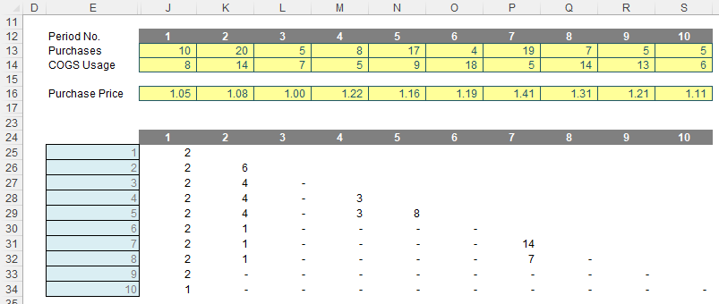
Do the values in rows 25:30 of the graphic look familiar?  This is keeping a running total of what inventory still remains.  As explained above, this is essential for working out costing and also useful for working out the age or remaining inventory, possible stockouts, etc.

In order to derive these numbers, I used a favourite function of mine…

Refresher on OFFSET (yet again!)

It seems every other article I bring this old chestnut up!  The syntax for OFFSET is as follows:

OFFSET(reference, rows, columns, [height], [width])

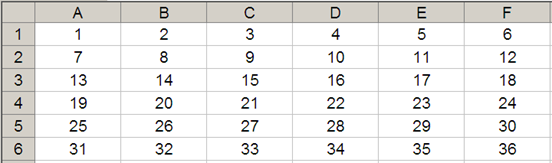
The arguments in square brackets (height and width) may be omitted from the formula, but I will need them here.  In its most basic form, OFFSET(reference, x, y) will select a reference x rows down (-x would be x rows up) and y columns to the right (-y would be y columns to the left) of the reference reference.  For example, consider the following grid:

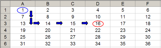
OFFSET(A1,2,3) would take us two rows down and three columns across to cell D3. Therefore, OFFSET(A1,2,3) = 16, viz.

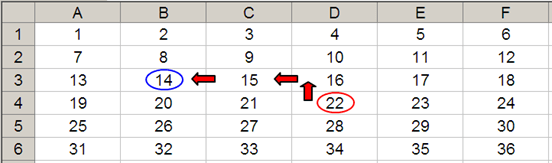
OFFSET may also take advantage of the height and width arguments.  If we extend the above formula to OFFSET(D4,-1,-2,-2,3), it would again take us to cell B3, but then we would select a range based on the height and width parameters.  The height would be two rows going up the sheet, with row 14 as the base (i.e. rows 13 and 14), and the width would be three columns going from left to right, with column B as the base (i.e. columns B, C and D). 

Hence, OFFSET(D4,-1,-2,-2,3) would select the range B2:D3, viz.

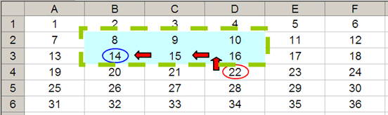
Note that OFFSET(D4,-1,-2,-2,3) = #VALUE! where dynamic arrays are not recognised, since Excel cannot display a matrix in one cell, but it does recognise it.  However, if after typing in OFFSET(D4,-1,-2,-2,3) we press CTRL + SHIFT + ENTER, we turn the formula into an array formula: {OFFSET(D4,-1,-2,-2,3)} (do not type the braces in, they will appear automatically as part of the Excel syntax).  This gives a value of 8, which is the value in the top left-hand corner of the matrix, but Excel is storing more than that.  This can be seen as follows:

• SUM(OFFSET(D4,-1,-2,-2,3)) = 72 (i.e. SUM(B2:D3))
• AVERAGE(OFFSET(D4,-1,-2,-2,3)) = 12 (i.e. AVERAGE(B2:D3)).

SUM(OFFSET) and OFFSET will both be useful here.

Returning to LIFO

Let’s revisit the grid:

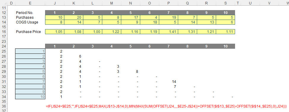
The formula in cell J25 is

=IF(J$24>$E25,"",
IF(J$24=$E25,MAX(J$13-J$14,0),
MIN(MAX(SUM(OFFSET(J24,,,,$E25-J$24))+OFFSET($I$13,,$E25)-OFFSET($I$14,,$E25),0),J24)))

Lovely.  I think this needs to be broken down!

Note that row 24 and the cells E25:E34 both denote the period number, so for eight periods we would have an eight by eight grid, and here, we have a 10 by 10 matrix.  Clearly, I cannot have any remaining inventory relating to periods later than the period presently being analysed, e.g. for Period 3, I could not take into account stock to be purchased in Period 4 or subsequently.  This rules out half of my matrix.  The formula

=IF(J$24>$E25,"", …

considers this.  If the period number to be analysed is if the period of usage the formula returns empty data (“”).  So far, so good.  The next period to consider is the actual period items are purchased and used (i.e. the leading diagonal of the grid), when the period number in the row and column are equal:

IF(J$24=$E25,MAX(J$13-J$14,0), …

In this situation, the remaining stock would be given by any excess of purchases over COGS usage, so for cell J25 this would equate to MAX(J$13-J$14,0).  The restriction is so that this number may not go negative.  It’s a simple calculation.  The issue is what follows!

MIN(MAX(SUM(OFFSET(J24,,,,$E25-J$24))+OFFSET($I$13,,$E25)-OFFSET($I$14,,$E25),0),J24)

Here, I have constructed a formula that is both replicable and scalable (this is why I have needed the OFFSET function). 

Given the recursive nature of the calculation, perhaps starting in Period 1 is not ideal as this situation cannot occur (this calculation only comes into force when we are looking to use prior period inventory to service current year usage – in the first period, by definition, we will have no prior inventory in this example).

Therefore, it is probably more appropriate to consider the copied down formula in cell J26 instead:

MIN(MAX(SUM(OFFSET(J25,,,,$E26-J$24))+OFFSET($I$13,,$E26)-OFFSET($I$14,,$E26),0),J25)

Here, let’s first consider the difference between the purchases made in Period 2 (cell K13, 20) and the COGS usage (cell K14, 14).  This would be given by the formula

K13-K14

Now the problem here is I want to copy this formula across the row so that it always references these cells:

$K13-$K14

OK, but when I copy the formula down a row I also need it to anchor to rows 13 and 14 respctively:

$K$13-$K$14

However, on the next row down I will want to reference rows L13-L14, etc.  I would have to write a different formula each row, which would become cumbersome: imagine coding a 20 year monthly model.  No thank you.  This is why I use

OFFSET($I$13,,$E25)-OFFSET($I$14,,$E25)

This uses the cell before the first purchased amount and the first used amount and then moves one column across for every row of the table (so Period 1 will use column J, Period 2 will use column K, etc.).  This now makes sense.

Word to the Wise

Apologies, it’s not the simplest concept we have ever discussed, but this is a common problem in financial modelling.  I wanted to show it for this reason – and because so many naysayers you cannot do this formulaically!

Some more advanced readers might consider using SUMPRODUCT and INDEX instead, or SUM and INDEX for those who have index to dynamic arrays.  This is because SUMPRODUCT cross-multiplies costs, and INDEX is not a so-called volatile function, which means it does not recalculate every time you press ENTER.

Given the name of my company is SUMPRODUCT, rest assured, dear reader, I have plenty of time for this function, but sometimes it slows down calculations.  Similarly, OFFSET may be volatile, but it also often calculates more quickly than INDEX, especially given you would need multiple INDEX expressions.  In larger models, you will find my formulae will calculate more quickly than using these alternatives – but it’s not wrong to use them instead.