“Array”, it’s such a simple word. It’s used all the time in normal speech - “I have an array of desserts for you to choose from”. Yet, when used in the context of Excel, for many it sparks panic. It seems confusing, it seems advanced.

This article aims to demystify arrays so you can feel confident knowing what they are and how they benefit you.

We will start somewhere simple, with something you already understand… ranges.

What is a range?

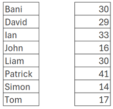
In simple terms, a range is a group of cells.

The formula in cell E2 is:

=XLOOKUP("Simon",A1:A8,B1:B8)

The formula uses XLOOKUP to lookup Simon from the range A1:A8 and return the corresponding value from the range B1:B8.

The result for Simon is 14.

The range references are made up of co-ordinates and an operator:

• The co-ordinates for the first range are: Column A, Row 1 to Column A, Row 8
• The co-ordinates for the second range are: Column B, Row 1 to Column B, Row 8
• The operator for both is a colon ( : ). This is known as the range operator. It creates a rectangular range which encompasses all the cells.

Ranges have visible presence on the worksheet. Therefore, we can see the values of "Bani", "David", "Ian", "John", "Liam", "Patrick", "Simon" and "Tom" are all included within the lookup_array argument. Also, 30, 29, 33, 16, 30, 41, 14 and 17 are included in the return_array argument.

That is ranges, now let’s look at arrays.

What is an array?

In simple terms, an array is a group of values.

The image above contains two grids with values, but we do not have row or column numbers.

These values don’t exist on the face of the worksheet. We don’t have any co-ordinates to refer to them. So, how can we perform an XLOOKUP using these values?

This brings us to an easy way to think about arrays. Arrays are a group of values which do not have cell co-ordinates.

Here is our XLOOKUP formula using the array values above (line breaks added for readability).

=XLOOKUP(
   "Simon",
   {"Bani";"David";"Ian";"John";"Liam";"Patrick";"Simon";"Tom"},
   {30;29;33;16;30;41;14;17})

Arrays have a specific syntax:

• Start and end with curly brackets ( { } ).
• Each column is separated by a comma ( , ).
• Each row is separated by a semi colon ( ; ).

NOTE: Depending on region settings, the array separators may be different.

In our example, the following are each columns containing 8 rows.

{"Bani";"David";"Ian";"John";"Liam";"Patrick";"Simon";"Tom"}

{30;29;33;16;30;41;14;17}

Using these arrays, XLOOKUP is still able to return the same result as before.

Let’s look at another example of using arrays:

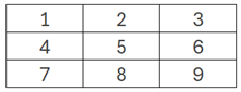
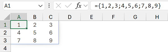
This grid of values has rows and columns; therefore, it can be expressed as an array as follows.

{1,2,3;4,5,6;7,8,9}

Pay close attention to the placement of the commas and semi-colons. Arrays must have the same number of columns in each row.

Converting between ranges and arrays

You are probably thinking it would be a big waste of time to hard-code array values to create a formula. Yes, I agree. Which is why we don’t hard code the values. Instead, we let Excel convert between ranges and arrays for us.

We’ve seen that ranges are a group of cells and arrays are a group of values.

Since cells contain values, and values are placed into cells, Excel switches between ranges and arrays automatically without us needing to think about it.

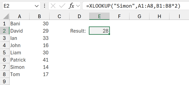
The formula in cell E2 is:

=XLOOKUP("Simon",A1:A8,B1:B8*2)

What’s happening in the formula?

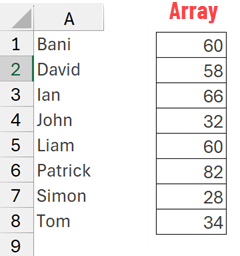
First, each value in the range B1:B8 is multiplied by 2. Therefore, changes from a group of cells (a range) into a group of values (an array).

In the background, Excel changes formula changes to:

=XLOOKUP("David",A1:A8,{60;58;66;32;60;82;28;34})

We noted earlier that a semi-colon is a row separator. So, we are forced to imagine what the rows and columns look like. Rather than picturing it in your mind, it may be easier to see the calculation as follows.

Excel performs the XLOOKUP on A1:A8, it finds Simon in the 7^th row and returns the 7^th row from the array. Therefore, the result is 28.

Excel didn’t care that it was mixing ranges and arrays. It simply converted the range into an array and performed the calculation as normal. We didn’t hard-code the array values, it happened automatically.

The opposite side of this, is when Excel converts arrays to ranges by returning results to the grid.

The formula in cell A1 contains an array:

={1,2,3;4,5,6;7,8,9}

By adding the equals sign at the start, Excel calculates the array and returns the values to the cells in the grid. The values now have co-ordinates which we can refer to; they have become a range.

Excel also handled this conversion from an array to a range automatically by returning the values to the grid.

In this section, we have seen that Excel automatically:

• Converts ranges to arrays through calculation
• Converts arrays to ranges by returning formula results

Therefore, we don’t need to hard-code values to work with arrays.

Array functions and array arguments

Most functions will happily work with ranges or arrays. Let’s use XLOOKUP as an example once again.

The first 3 arguments of XLOOKUP are:

• Lookup_value: The value to search for
• Lookup_array: The array or range to search
• Return_array: The array or range to return

Did you notice the words used to describe the lookup_array and return_array? … “array or range”. This means Excel is happy with either a range or an array.

Since arrays don’t have visible presence on the grid, we can easily reshape them using functions.

Excel has lots of array shaping functions, VSTACK, HSTACK, CHOOSECOLS, CHOOSEROWS, TAKE, DROP, TOROW, TOCOL, and more. You can learn more about these functions in a previous article.

These functions select, remove, combine and reshape values from multiple ranges or arrays into a single array. Which means, we can use array functions to pre-shape values before using them in other functions.

You might be thinking, “So what, is this actually useful?” Let’s take a look at an example.

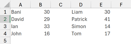
In the screenshot above, we have multiple ranges. The names are in A1:A4 and D1:D4. The values are in B1:B4 and E1:E4.

Using ranges alone, we can’t use XLOOKUP, because we have multiple ranges for each column. However, we can combine multiple ranges into an array, which we then use inside XLOOKUP.

Let’s use the VSTACK function. It stacks arrays or ranges on top of each other and creates an array of all the values.

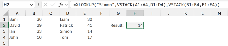
The formula in cell H2 is:

=XLOOKUP("Simon",VSTACK(A1:A4,D1:D4),VSTACK(B1:B4,E1:E4))

The first VSTACK function takes ranges A1:A4 and D1:D4 and turns them into a single array of:

{"Bani";"David";"Ian";"John";"Liam";"Patrick";"Simon";"Tom"}

The second VSTACK function takes ranges of B1:B4 and E1:E4 and turns them into a single array of:

{30;29;33;16;30;41;14;17}

Which means, the XLOOKUP calculation changes to:

=XLOOKUP(
   "Simon",
   {"Bani";"David";"Ian";"John";"Liam";"Patrick";"Simon";"Tom"},
   {30;29;33;16;30;41;14;17})

This is exactly the same as the array example we saw earlier in the article, but we didn’t hard code any values, Excel handled this for us.

By combining multiple ranges into arrays using VSTACK, XLOOKUP can return the result from multiple tables. This is the magic of arrays.

Most functions work with arrays. Therefore, if necessary, we can use the array functions named above to pre-shape any values into arrays before using them in other functions.

NOTE: The most notable functions which don’t work with arrays are the conditional aggregator functions: SUMIF, SUMIFS, AVERAGEIF, AVERAGEIFS, etc.

What about dynamic arrays?

We’ve looked at arrays, and seen they are a group of values that can be hard-coded or created through calculation.

You may also have heard the term “dynamic array”. If you thought “array” sounded confusing, adding the word “dynamic” at the start just adds to that confusion. So, let’s try to simplify that.

Arrays come in two forms, static (also known as constant arrays) and dynamic.

If we were to enter the following array into a cell, it would create a column with numbers 1 to 4.

={1;2;3;4}

It would always calculate that result. It could never calculate anything else. The result would be static.

The SEQUENCE function creates arrays with lists of numbers. If we were to use the following, it would also create a column with numbers 1 to 4.

=SEQUENCE(4)

It would always calculate that result. It could never calculate anything else. Just like hard coded array values, the result would be static.

However, instead of using 4, let’s use cell A1.

=SEQUENCE(A1)

How many rows are in the array? Excel has no idea until it calculates and looks in cell A1. It could be 4 it could be 1,000. This is known as a dynamic array because the size of the array can change at each calculation.

And, that’s it. A dynamic array is just a calculation in which the number of values is unknown until the calculation is performed.

Conclusion

In this article, we have seen that ranges are a group of cells and arrays are a group of values. Excel automatically switches between ranges and arrays, so we don’t have to think about it.

Ranges in themselves are limited because they must exist on the grid. But we can turn ranges into arrays through calculation. This allows us to use array functions to pre-shape values before we use them in other functions, which provides more flexible ways to solve Excel problems.

If you’ve not done so already, take a look at the array shaping functions (VSTACK, HSTACK, CHOOSECOLS, CHOOSEROWS, TAKE, DROP, TOROW, TOCOL) and consider how you can use them to pre-shape the values into arrays before using them in other functions.