Principle 14 of the 20 Principles for Good Spreadsheet Practice is “Avoid using fixed values within formulas”. Therefore, the inputs we use in our formulas will nearly always come from cell ranges, rather than static values.

Yet, I have never been taught how to use cells and ranges in Excel, and I doubt you have either. In fact, as Excel users it’s surprising how little time we spend learning about what could be Excel’s most used feature.

Most users think ranges are simple; select some cells, include a colon, throw in a few $ signs, and that’s it. Well, there is a lot more to ranges than that, and in this article, we are going to cover only one aspect; Range functions.

What is a range function?

A range function is any function which returns a range as the result.

Let’s look at an example:

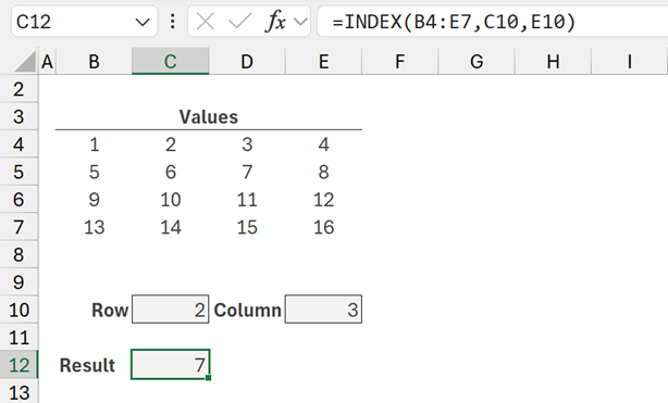
The formula in cell C12 is:

=INDEX(B4:E7,C10,E10)

We can be forgiven for thinking the formula is looking at the range B4:E7, it finds row 2 (the value from C10) and column 3 (the value from E10) and returns the value 7 - after all, that’s what Excel is showing us.

However, what Excel doesn’t show us is that this is a two-stage calculation.

Stage	Calculation	Result
1	=INDEX(B4:E7,C10,E10)	=D5
2	=D5	7

Excel only shows us the result after Stage 2, we don’t get to see the result of Stage 1.

However, since INDEX is a function which returns a range, it means we can use the result of stage 1 as a range reference.

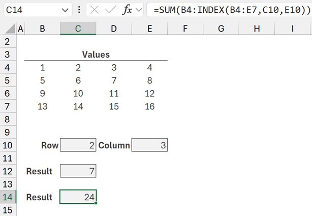
The formula in cell C14 is:

=SUM(B4:INDEX(B4:E7,C10,E10))

This might look strange, so let’s step through it.

Stage	Calculation	Result
1	=SUM(B4:INDEX(B4:E7,C10,E10))	=SUM(B4:D5)
2	=SUM(B4:D5)	24

INDEX returns D5 as a range reference. This is used to create the full reference of B4:D5 which is used in the SUM function.

If we change the values in C10 and E10, it creates ranges of different sizes. The range size is dynamic. Therefore, this is known as a dynamic range.

In our SUM example, there are two cell references that form the full range reference. And we could use a range function for both of them. 

In the formula below we use two INDEX functions, one on each side of the colon. They are each returning a range reference and forming a new range.

Stage	Calculation	Result
1	=SUM(INDEX(B4:E7,1,1):INDEX(B4:E7,2,3))	=SUM(B4:D5)
2	=SUM(B4:D5)	24

Which functions are range functions?

INDEX is not the only range function, there are many more. We can use any of the following functions as substitutes for a static range reference.

Note: All the examples below are based on the screenshot above.

CHOOSE

Uses a number to return the nth value from the a list of values.

Example	Result
=CHOOSE(2,B4:B7,C4:C7,D4:D7,E4:E7) The first argument of CHOOSE determines which value to return. As the first argument is 2, the second range in the list is returned.	=C4:C7

DROP

Excludes a specified number of rows or columns from the start or end of a range or array.

Example	Result
=DROP(B4:E7,2) The second argument of DROP shows we will remove 2 rows from the top of the range.	=B6:E7

IF

Compares a value to a condition and returns a value based on whether the condition is true or false.

Example	Result
=IF(0>1,B4:C7,D4:E7) 0 is not greater than 1, therefore the FALSE path is taken.	=D4:E7

IFS

Returns the value which corresponds to the first TRUE result.

Example	Result
=IFS(0>1,B4:B7,1>1,C4:C7,2>1,D4:D7) The first test which returns true is 2>1, therefore the result returned is the next argument.	=D4:D7

INDEX

Returns the value from a range or array based on the row and column number.

Example	Result
=INDEX(B4:E7,2,3) This uses B4:E7 and returns the value in row 2 and column 3.	=D5

INDIRECT

Returns the reference specified by a text string.

Example	Result
=INDIRECT("D5") Creates a range reference based on the text value.	=D5

OFFSET

Returns a reference to a range that is a specified number of rows and columns from a start point and with a specified height and width.

Example	Result
=OFFSET(B4,0,2,4) Starting on cell B4, move 0 rows, 2 columns and create a range 4 rows high.	=D4:D7

SWITCH

Compares a value against a list of values and returns the result corresponding to the first matching value.

Example	Result
=SWITCH(TRUE,0>1,B4:B7,1>1,C4:C7,2>1,D4:D7) The first test which returns TRUE is 2>1 therefore the result returned is the next argument.	=D4:D7

TAKE

Returns a specified number of rows or columns from the start or end of a range or array.

Example	Result
=TAKE(B4:E7,2) The second argument of TAKE shows we will take the first 2 rows from the top of the range.	=B4:E5

TRIMRANGE

Excludes all empty rows and/or columns from the outer edges of a range or array.

Example	Result
=TRIMRANGE(A4:F8) The range which includes values is B4:E7, the other cells are blank.	=B4:E7

Note: At the time of writing TRIMRANGE is only available in the Excel 365 beta channel.

XLOOKUP

Searches a value and returns the item corresponding to the first match it finds from another range or array.

Example	Result
=XLOOKUP(5,B4:B7,C4:C7) Find 5 in B4:B7, then return the corresponding value from C4:C7.	=C5

When a range function is not a range function

While the functions above are capable of returning ranges, they do not always do so.

With the exception of INDIRECT which creates a range reference based on text, for the remaining functions, to return a range, the inputs for the return value must also be a range.
In the example below the return_array for XLOOKUP comes from C4:C7, therefore it will return a range.

=XLOOKUP(5,B4:B7,C4:C7)

However, what happens if the return_array were not a range, but an array?

=XLOOKUP(5,B4:B7,{3;7;11;15})

The formula above is valid. However, 3, 7, 11 and 15 are numbers and do not have range positions. Therefore,  for this formula, XLOOKUP cannot return a range reference.
This also means we cannot perform a calculation on the range prior to evaluation inside the function.

In the function below C4:C7 is multiplied by 100.

=XLOOKUP(5,B4:B7,C4:C7*100)

By performing the calculation, C4:C7 is transformed into an array with the following values {300;700;1100;1500}. As a result, XLOOKUP cannot return a range, because the return_array argument is now an array.

An easy way to identify if a function is returns a range, is to wrap the function inside ISREF.

Example	Result
=ISREF(XLOOKUP(5,B4:B7,C4:C7))	TRUE
=ISREF(XLOOKUP(5,B4:B7,C4:C7*100))	FALSE

Where to use range functions?

We have seen what range functions are and how they work. We have also seen them used to create dynamic ranges for calculation. But are they useful for anything else?

Most Excel features will happily work with ranges or arrays, but some only work with ranges. In these circumstances we can often use range functions to create dynamic calculations.

Let’s take a look at some features which require ranges.

Conditional aggregator IF/IFS functions

The conditional aggregator functions are SUMIF, SUMIFS, COUNTIF, COUNTIFS, AVERAGEIF, etc.

Let’s use SUMIFS as an example. SUMIFS has arguments of:

• Sum_range
• Criteria_range1
• Criteria1
• Criteria_range2
• Criteria2
• … etc.

The Sum_range, Criteria_range1 and Criteria_range2 must all be ranges, they do not work with arrays.

If we want to dynamically select which column to use for the sum_range, we can use a range function.

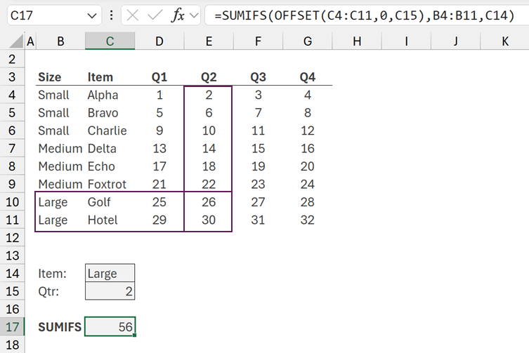
The formula in cell C17 is:

=SUMIFS(OFFSET(C4:C11,0,C15),B4:B11,C14)

The OFFSET function creates a dynamic range to select Quarter 2 (cells E4:E11). This is used inside the SUMIFS to only calculate the Large sizes.

Data Validation Lists

Data validation lists can use values from ranges, but not from arrays. Therefore, we can use range functions to dynamically select the values to display in a Data validation list.

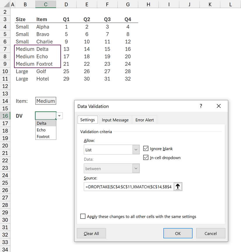
 Cell E16 contains a data validation list.

The formula used for the data validation List is:

=DROP(TAKE($C$4:$C$11,XMATCH($C$14,$B$4:$B$11,,-1)),XMATCH($C$14,$B$4:$B$11)-1)

This formula uses TAKE and DROP to return the range for the Items where the Size is Medium.

If C14 were Small or Large the data validation list would only display the corresponding items.

Charts

Excel charts can be linked to ranges for dynamic presentation.

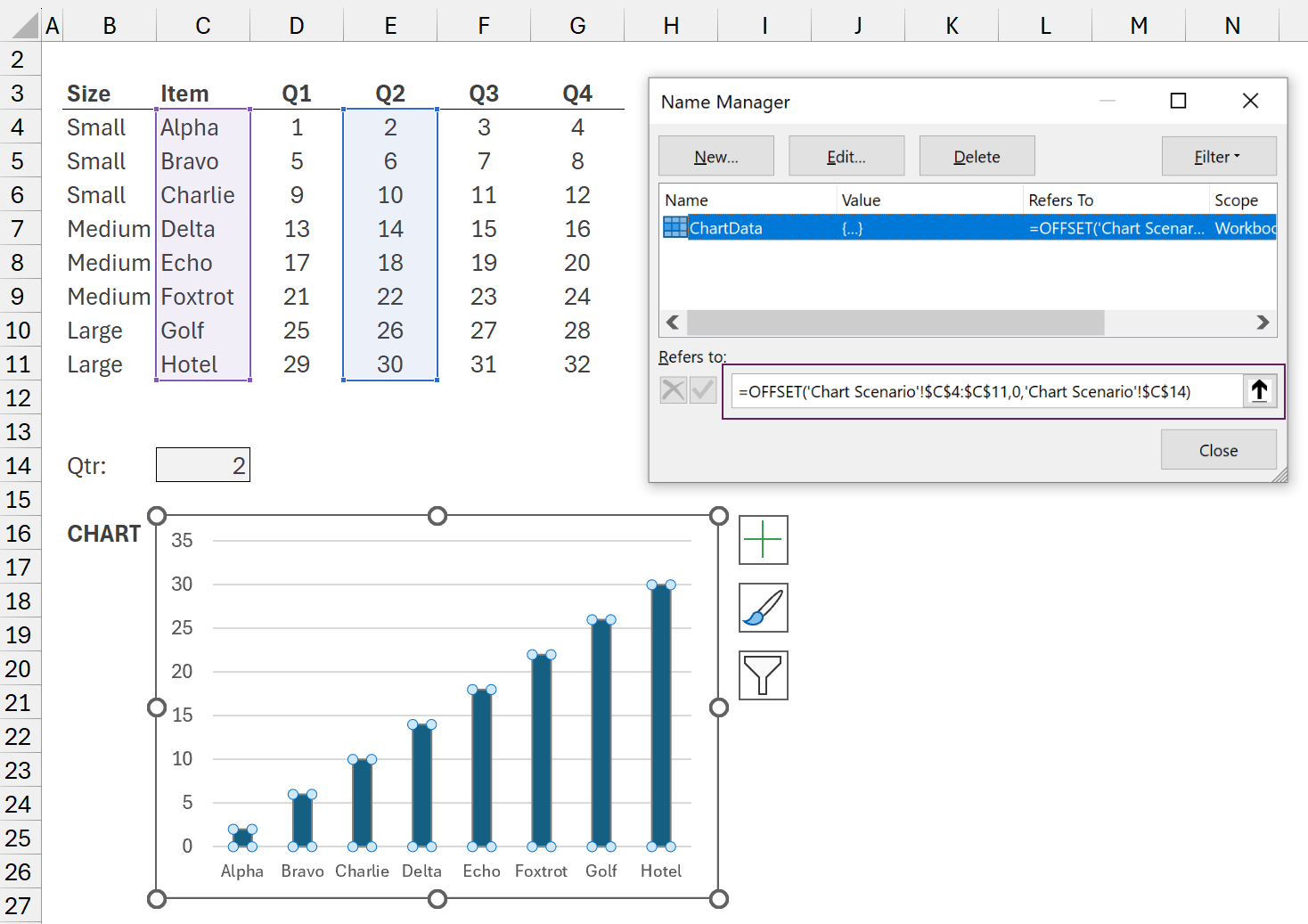
We created a named range called ChartData. This includes the following formula:

=OFFSET('Chart Scenario'!$C$4:$C$11,0,'Chart Scenario'!$C$14)

Because C14 is 2, OFFSET returns the data from Q2 (cells E4:E11).

We then use the named range in the chart source. Therefore, the range for the chart is dynamic, it is based on a result of a range function.

If the value in C14 changes, the chart range updates dynamically.

Conclusion

In this article, we have seen there are special functions which, when provided with a range as an input, are able to return a range output.

We can use this range output in place of static range references. These create dynamic ranges which move and resize upon calculation.

While commonly used for flexible on grid calculations, they are also a useful tool for working with many Excel features, such as data validation and charts.